When you read about linear mixed models, you will quickly come across the terms ‘fixed factors’ and ‘random factors’. What do these terms refer to? Why are they so important to understand when first learning about linear mixed models?

Fixed factors

Most students and researchers should be familiar with fixed factors. Fixed factors are those that we we traditionally would is in an analysis of variance (ANOVA) or an analysis of co-variance (ANCOVA). Fixed factors are categorical or classification variables that are of interest to the study. In our previous example about the effect of consuming a shot of maple syrup on a person’s ability to perceive the weight of a lifted object, we measures ‘pre’ and ‘post’ maple syrup ingestion. We also compared between taking a shot of maple syrup and taking a shot of water (our control condition).
Thus, in this study, time (pre, post) and shot (syrup, water) are both fixed factors.

Levels of a fixed factor are chosen so that they represent specific conditions, and they can be used to define specific contrasts that we are interested in.

Lets consider a second example: a randomised clinical trial looking at the effect of maple syrup on bone strength in the elderly. We randomised 100 participants to either ingest a 20ml of maple syrup (treatment group) or 20ml of tinted, thickened flavoured water (placebo group) morning and night for 6 months. Bone density measures were taken at baseline and after 6 months. In this study, we are interested in whether bone density was better at the 6-month mark in participants in the syrup group compared to the placebo group. Thus, we would compare the 6-month data and include a fixed factor for intervention (syrup vs placebo) and fixed factor for our included co-variate of baseline bone density scores (more on this in a later blog post).

Random factors

The inclusion of both fixed factors and random factors are what make linear mixed models ‘mixed’; they include a mixture of fixed factors, like those described above, as well as random factors.

As a non-statistician, I know what a random factor is (or at least I think I do), but I don’t have a simple explanation of what it is. Thus, I will try to explain why these factors are required and hopefully what they are will become evident.

What if we simply accounted for each participant in the model?

In his book “Applied Longitudinal Data Analysis for Medical Science: A Practical Guide”, Jos WR Twisk provides a simple and clear explanation of why we might need a random factor in our linear regression model. I will use a fictive (yes, maple-syrup based) example to work through the logic. We were able to obtain another grant from the Maple Syrup Consortium, this time to investigate whether sleeping on a maple-syrup infused pillow increased a person’s happiness.
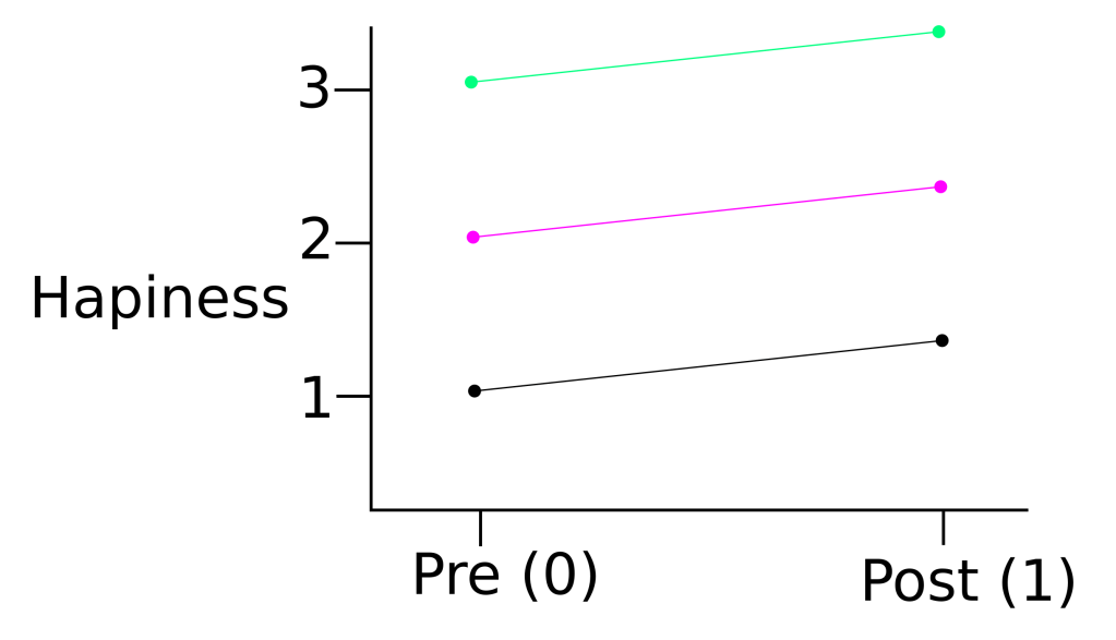
In this study, we measured peoples perceived happiness at the start of the study, and 2 months later, after sleeping on their maple pillow every night. An example of data from three of the study participants is presented in Figure 1.

If the data points in the present study were truly independent, we could use simple linear regression to determine the effect of sleeping with a maple pillow on happiness.

Here, are our observations of the outcome at time , is the intercept, is the regression coefficient for the fixed factor , and is the error for time .

But there is a major problem! A key assumption of simple linear regression is that the observations of independent of one another. In the present example, pairs of data points in the ‘pre’ and ‘post’ periods come from the same participants; these two data points are not independent.

A simple solution is to extend our regression model to include an extra regression coefficient for each participant. In the current example, we have three participant: A, B, C. Thus, we can use dummy coding of two fixed factors to account for these three participants:

	Participant 1	Participant 2
A	0	0
B	1	0
C	0	1

We can then use these additional fixed effects to account for the dependence of data within participants. Specifically, we include terms that allow each study participant to have a different intercept.

In the present example, let’s imaging that we fit our model and we obtained the following coefficients:

Now, let us consider the case of Participant A (black line and dots). If we want to model their data at the ‘pre’ time point,

would be because time is coded as either (pre) or (post). Also, and would be set to , given our dummy coding shown in the above table.

If we want to model their data at the ‘post’ time point, we would use the following equation:

Now comes the cool part! What if we wanted to model the pre-post data for Participants B (magenta) and C (lime green)?
Easy, simply use to correct dummy codes.

Participant B – pre

By setting to and to $0$, we allow Participant B to have their own intercept (i.e. value at ‘pre’, given that ‘pre’ is coded as along the x-axis).

Participant B – post

Participant C – pre

Participant C – post

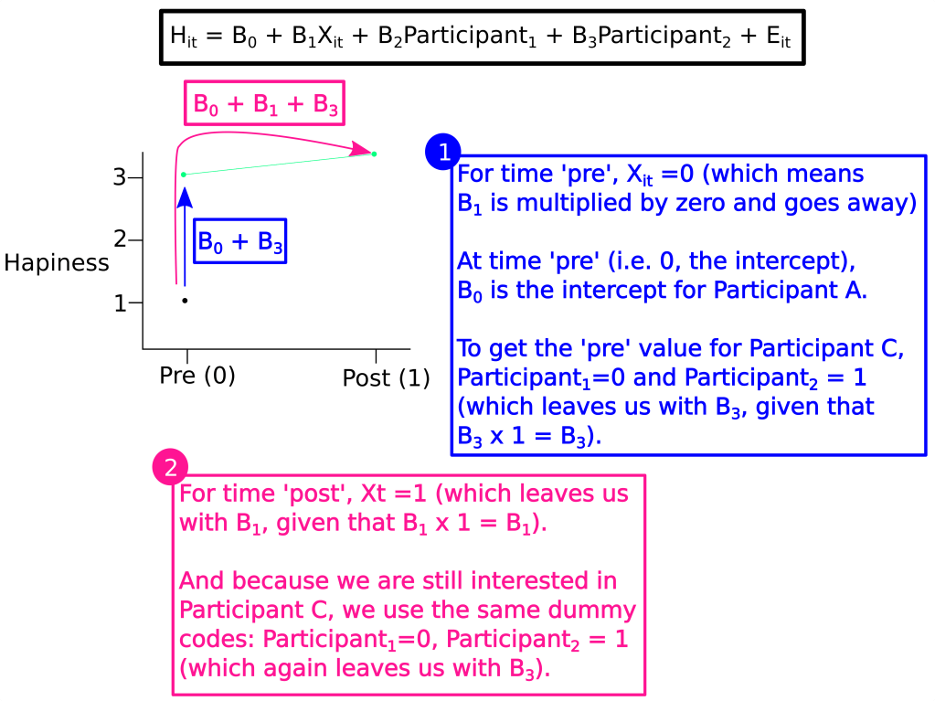
In case you did not follow what was going for Participant B and C, Figure 2 provides a visual explanation of how the ‘pre’ and ‘post’ data for Participant C are modeled.

What if we included only one additional random factor instead?

Given the popularity of our maple-syrup infused pillows, Image if we got another grant, but this time for maple-syrup infused nappies! What a great idea. But, because of the odour that we are fighting against, we will probably need a much larger sample size. Imagine if we had to recruited 100 babies. That would mean that we would need to include 99 baby specific coefficients to account for the dependency of their ‘pre-post’ data.
That is a lot of coefficients! Not only is this inefficient and cumbersome to work with, it will also result in less powerful statistical test. Is there a better solution?

Yes! We are not actually interested in the coefficient associated with baby Billy, Bailey, Brandon or Beatrice; we simply have to account for the dependence in their data. To do this, we include a random factor. In the example we used above (i.e. maple pillows), what we want is a random factors that accounts for the different intercepts across study participants. And that is exactly what we can use: a random intercept.

More on this in the next post.

What if clusters have different patterns of responses, can we also account for this as well?

Let’s return to our example from the previous post, where we considered the effect a school has on student responses.
Specifically, we noticed that students from the same school tended to response more similarly than students from different schools. Here is the relevant figure from the previous post:

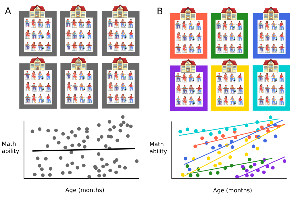
Hopefully you can see that, here too, we probably want to include a random intercept term to account for the school-level effect on student maths ability. But there is another thing to notice: the slope of the plotted lines differ across schools. This means that, at least in the example we have here, the effect of age in months has on maths ability differs across schools. While in some schools, each extra month of age might result in a 5 point increase in maths ability,
the same extra month might be associated with a 10 point increase in maths ability in a different school.

Again, we are no particularly interested in the specific schools tested and their specific intercepts and slopes. Rather, we want to account for this dependency and be able to draw conclusions for the entire population of schools. This means that, instead of including several regressions coefficients to account for the different slopes across schools similar to what we had to do by including in our example above), we can include what is called a random slope in our model to allow the pattern of responses (i.e. their slope) to differ cross schools/participants, etc. We will go into more detail about random slopes in our next post.

Summary

Linear mixed models include a mixture of fixed and random factors. Although the present post only provided a cursory introduction, it is important to know that several random factors can be included in a model, and these models can cross different levels (e.g. students, schools, districts) of a given model. There is much more to say about random factors, some of which will be presented in the next post.