In a previous post we learned how to perform an independent t-test in R to determine whether a difference between two groups is important or significant. In this post we will learn how to perform the same test using the Python programming language. Along the way we will learn a few things about t distributions and calculating confidence intervals.

Get our data out of R and into Python

The first thing we need to do is save the data we created in R in a format that we can easily read in Python. In this example we will save the data to a csv file (i.e., comma-separated values). Remembering that our variable containing all the data was called data, we can run the following command in R to save a csv version of our data:

write.table(data, file = "data.csv",row.names=FALSE, na="", col.names=TRUE, sep=",")

Great! We now have a copy of our beef and pork data saved in a file called data.csv. The next thing we need to do is read this data into Python. We will be using the dataframe data type to store our beef and pork data in Python. This data type is part of the Pandas library, so we will have to import Pandas before we can use it to import our data.csv file:

import pandas
data = pandas.read_csv('data.csv')

Great! We now have the data in Python and we are ready to perform our independent t-test.

Independent t-test in Python

It is quite simple to perform an independent t-test in Python.

from scipy.stats import ttest_ind
ttest_ind(data.value[data.names == 'beef'],data.value[data.names == 'pork'])

We first import the relevant function from the stats portion of the scipy library. We then run our independent t-test using the following command: ttest_ind(group1_data, group2_data).

For our data, running this command outputs:

Ttest_indResult(statistic=2.3774364252931681, pvalue=0.020751512609572479)

Great! We got the same answer as we did with R: the t-value is 2.37 and the p-value is 0.02.

But something is missing! If you remember the previous post, the output of the independent t-test performed in R returned the mean value of each sample as well as the 95% confidence interval of the difference between the two groups. Because these bits of information are important for reporting and interpreting our results, we will learn how to compute them using Python.

Calculating the mean [95% confidence interval] difference between two independent groups in Python

The first thing to do is calculate the mean difference between the two groups. This is easily accomplished using the .mean() method of the dataframe data type. Don’t worry to much if you don’t know what a method is, you can still follow along and non will be the wiser.

mean_beef = data.value[data.names == 'beef'].mean()
mean_pork = data.value[data.names == 'pork'].mean()
diff_mean = mean_beef - mean_pork

That was pretty simple. The mean difference betwen groups is 91.57 kg.

The next thing we need to do is calculate the 95% confidence interval of this difference. To do that, we will calculate what is known as the margin of error or MoE. This is a fancy term to say one side of the confidence interval.

The formula for the margin of error is: MoE = t.95(df) * std_N1N2 * (1/sqrt(N))

The first term in the formula is the t component, which is based on the degrees of freedom associated with our data (df = N1 + N2 - 2). Because our data comes from 30 beef and 30 pork, our df = 58 (i.e., 30 + 30 -2).

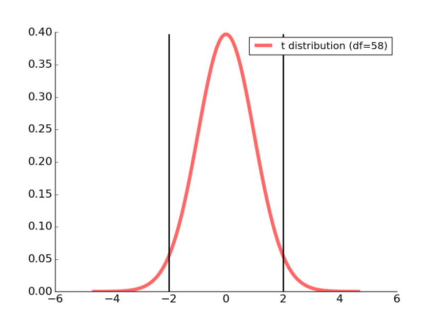
The t component of the formula corresponds to the t-value associated with our 95% cut-off. We can find this t-value by looking at a t-distribution and seeing what number corresponds 97.5% (because 2.5% to 97.5% corresponds to 95% of the data). However, it is important to know that there are many t-distributions. We can generate a different t-distribution for any value of df. The larger the value of df, the more the t-distribution will resemble the normal distribution.

Our t distribution associated with a df of 58 is plotted as a red line in the figure below.

Figure 2: The two black lines correspond to the 95% confidence interval for this t-distribution.

We can calculate the t-value associated with our 95% cut-off using the percent point function from Student’s t in scipy.stats:

from scipy.stats import t
t_val = t.ppf([0.975], df)

Running this code informs us that the t-value is 2.00171748, which we can see on the right half of the t-distribution plotted above.

The next portion of the MoE formula is std_N1N2. This corresponds to the average standard deviations between groups.

from math import sqrt
N1 = 30
N2 = 30
std1 = data.value[data.names == 'beef'].std()
std2 = data.value[data.names == 'pork'].std()
df = (N1 + N2 - 2)
std_N1N2 = sqrt(((N1 - 1)*(std1)**2 + (N2 - 1)*(std2)**2) / df) 

The final component of the MoE formula is (1/sqrt(N)). This can be computed as follows:

sqrt(1/N1 + 1/N2)

We now have everything we need to calculate our MoE.

MoE = t.ppf(0.975, df) * std_N1N2 * sqrt(1/N1 + 1/N2)

Our MoE is 77.1.

Putting it all together

Below I have written out the code as I would us it in my own data analysis program. I always include print statements so that I have a nice summary of the main values I calculated.

import pandas
from scipy import stats
from math import sqrt
from scipy.stats import t

# Import data
data = pandas.read_csv('data.csv')

# Run independent t-test
ind_t_test = stats.ttest_ind(data.value[data.names == 'beef'],data.value[data.names == 'pork'])

# Calculate the mean difference and 95% confidence interval
N1 = 30
N2 = 30
df = (N1 + N2 - 2)
std1 = data.value[data.names == 'beef'].std()
std2 = data.value[data.names == 'pork'].std()
std_N1N2 = sqrt( ((N1 - 1)*(std1)**2 + (N2 - 1)*(std2)**2) / df) 

diff_mean = data.value[data.names == 'beef'].mean() - data.value[data.names == 'pork'].mean()
MoE = t.ppf(0.975, df) * std_N1N2 * sqrt(1/N1 + 1/N2)

print('The results of the independent t-test are: \n\tt-value = {:4.3f}\n\tp-value = {:4.3f}'.format(ind_t_test[0],ind_t_test[1]))
print ('\nThe difference between groups is {:3.1f} [{:3.1f} to {:3.1f}] (mean [95% CI])'.format(diff_mean, diff_mean - MoE, diff_mean + MoE))

Running this code prints out the following:

The results of the independent t-test are: 
    t-value = 2.377
    p-value = 0.021

The difference between groups is 91.6 [14.5 to 168.7] (mean [95% CI])

Thankfully, these are the same values we obtained using R in our previous post.

Summary

Compared to our previous experience with R, it was more work getting all the output values with Python. However, we learned a lot about t-distributions and margins of errors.

If you regularly use Python, you might prefer to do all your work there. Hopefully you will keep this post in mind the next time you have to run an independent t-test!