Calculating sample size using precision for planning

Most sample size calculations for independent or paired samples are performed based on power to detect an effect of a certain size, assuming there’s no effect. Instead, Cumming and Calin-Jageman recommend that readers plan studies to detect precise effects.
The 95% confidence interval (CI) indicates precision about effects. Therefore, it is possible to plan studies to detect narrow 95% CIs about effects, instead of plan studies to detect the existence of effects.
How are 95% CIs used to perform sample size calculations? The margin of error (MOE) is one side of a CI. For a single group design, the MOE is expressed as:

with sample size 


where 

Cumming’s text provides sample size calculation formulas for two independent groups and paired comparisons, assuming known
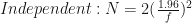
where 
>>>:
z = 1.96
fractions = [0.4, 0.5, 0.6] # fractions of population SD
for f in fractions:
print('\nFraction of population SD: {}'.format(f))
# Two independent groups
N = 2 * (z/f)**2 # z assumes population SD is known
print('N in *each* group: {:.2f}'.format(N))
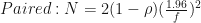
# Paired groups
rho = 0.4 # correlation in population between the two measures
N = 2 * (1 - rho) * (z/f)**2
print('N of paired group: {:.2f}'.format(N))
>>> Fraction of population SD: 0.4
>>> N in *each* group: 48.02
>>> N of paired group: 28.81
>>> Fraction of population SD: 0.5
>>> N in *each* group: 30.73
>>> N of paired group: 18.44
>>> Fraction of population SD: 0.6
>>> N in *each* group: 21.34
>>> N of paired group: 12.81
Summary
It is possible to use precision for planning to calculate sample size to detect the width of the confidence interval. This encourages readers to think about size and precision of effects. Cumming’s text provides more details to calculate sample size as above when population standard deviation is not known.
References
Cumming G (2012). Understanding the New Statistics: Effect Sizes, Confidence Intervals, and Meta-Analysis. Routledge, East Sussex. p 357.
Cumming G & Calin-Jageman R (2017). Introduction the New Statistics: Estimation, Open Science & Beyond. Routledge, East Sussex.

Is there an R script that can do what the Python script does?
Or would one need to run Python in R?
LikeLike
Thanks for your comment.
I’m not aware of a specific R package that calculates sample size for precision, but Cumming and Calin-Jageman refer readers to the statistical programs jamovi (built on R) and JASP which perform estimation statistics. There may be related modules in these programs to calculate sample size.
LikeLike
Thanks Joanna! I’m an R and Jamovi user. So I may be able to find a solution between the two. I can try to share it here if I find it.
LikeLike
Thanks Nick, yes please do share pointers. Cheers
LikeLike