In statistics, we often want to fit a statistical model to be able to make broader generalizations. An important type of statistical model is linear regression, where we predict the linear relationship between an outcome variable and a predictor variable. In this post we will learn how to perform a simple linear regression in R. See our previous post for a bit of background on how linear regression works.

Nothing to wine about

When I was growing up, my dad was always making homemade wine. From what I understand, there were some successes as well as some failures (“C’est de la piquette!”). One thing I learned was that you could use simple equipment to make measurements as the wine fermented. You can use a hydrometer to test the gravity of the wine mixture (an indirect measure of alcohol formation as the wine ferments). If you are very keen, you can use a pycnometer to more precisely measure the alcoholic strength of the wine. But again this device does not directly measure the alcoholic content of the wine; it measures the density of the wine. Therefore, we should be able to predict the alcohol content of a wine (a measure that would require real laboratory equipment) by taking a measure of its density.

I found an interesting dataset on the internet about various measures taken from thousands of wines. To simplify things, I took a random sample of 200 white wines; this smaller dataset is available for download here.

Plotting the relationship between wine alcohol content and wine density

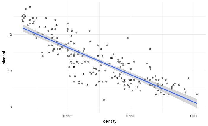
It is always a good idea to first plot our data. The R code below imports that data and generates a scatterplot with a trendline between the density of the white wines (x-axis) and the alcohol content of the white wines (y-axis).

# Import ggplot2 plotting library
library(ggplot2)

# Import data (change path to where you have downloaded and save white.csv)
setwd("~/Desktop/regression")
white <- read.csv("white.csv", header=TRUE)

# Generate simple scatter plots with trend lines
ggplot(white, aes(density, alcohol)) +  
       geom_point(alpha=0.5) +  
       geom_smooth(method = "lm") +  
       theme_minimal()

We can see that there is a strong linear relationship between the density of the white wines and their alcohol content. Because the line is pointing downwards, we know that it will have a negative slope. This means that as the density of a wine increases, its alcohol content decreases.

Testing the linear regression

We will use the car library (Companion to Applied Regression) to compute our linear regression in R. Specifically, we will use the lm() function to fit our linear model.

The code below indicates that we create our model object alcohol1 by specifying that our outcome variable (alcohol) is to be predicted from our predictor variable (density).

library(car)
alcohol1 <- lm(alcohol ~ density, data=white)

We can see the results of our model by call the summary() function on our model object.

summary(alcohol1)

Call:
lm(formula = alcohol ~ density, data = white)

Residuals:     
    Min       1Q   Median       3Q      Max 
 -2.01860 -0.47670  0.02203  0.50253  1.94904 

Coefficients:            
             Estimate Std. Error t value  Pr(>|t|)    
(Intercept)  384.19     18.00     21.34   2e-16 ***
density      -375.92    18.11    -20.75   <2e-16 ***
---
Signif. codes:  0 ‘***’ 0.001 ‘**’ 0.01 ‘*’ 0.05 ‘.’ 0.1 ‘ ’ 1

Residual standard error: 0.7063 on 198 degrees of freedom
Multiple R-squared:  0.6851,    Adjusted R-squared:  0.6835 
F-statistic: 430.7 on 1 and 198 DF,  p-value: < 2.2e-16

R-squared. There is a lot to take in here. As we saw in our previous post, we usually want to know how well our model fits the data. We can determine this by looking at the value of . In our white wine example, we see that . This means that, of the total variability in the simplest model possible (i.e. mean alcohol) calculated as the total sum of squares, 69% of it was accounted for by our linear regression model.

F-test and p-value. Although regression analysis always returns a model, it does not mean the model is good (i.e. explains a large portion of the overall variability in the data). Therefore, we want to also look at the result of the F-test. Our F-statistic is 430.7 with 1 and 198 degrees of freedom. R informs us that this is associated with a very small p-value. Thus, the probability of observing such a large F-statistic if the model accounted for no variability is very small.

Individual predictors. When a model has a single predictor, a significant F-test indicates that the predictor significantly predicts the outcome variable. However, this is not true in multiple regression (which we will tackle in a later blog). Also, the coefficients associated with our model provide important information.

In the summary output above, R returns coefficients for the intercept of our linear model (sometimes referred to as and our predictor variable (i.e. ). We can see that the coefficient associated with density is highly significant (a t-test indicates it is significantly different from zero). Together, these coefficients describe our model, the regression line plotted over our data. Thus:

alcohol = + * density + error

alcohol = * density + error

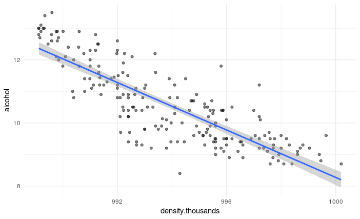
While this equation describes our model and regression line, it is a little hard to interpret. It is telling us that for a 1 unit change in density, alcohol decreases by 375.9. To obtain obtain a more useful coefficient, we can multiply our density data by 1000 and rerun the analysis. The revised plot and summary() are presented below.

Call:
lm(formula = alcohol ~ density.thousands, data = white)

Residuals:
     Min       1Q   Median       3Q      Max 
-2.01860 -0.47670  0.02203  0.50253  1.94904 

Coefficients:
                   Estimate Std. Error t value Pr(>|t|)    
(Intercept)       384.19107   18.00176   21.34   <2e-16 ***
density.thousands  -0.37592    0.01811  -20.75   <2e-16 ***
---
Signif. codes:  0 ‘***’ 0.001 ‘**’ 0.01 ‘*’ 0.05 ‘.’ 0.1 ‘ ’ 1

Residual standard error: 0.7063 on 198 degrees of freedom
Multiple R-squared:  0.6851,    Adjusted R-squared:  0.6835 
F-statistic: 430.7 on 1 and 198 DF,  p-value: < 2.2e-16

alcohol = + * density + error

alcohol = 384.2 + -0.38 * density + error

From this new output, we can see that a change of one-thousands in white density (i.e. 0.001) is associated with a reduction in alcohol of 0.38.

Summary

We have seen how to perform linear regression on a simple dataset. As the figures and results show, the density of white wine has a strong linear relationship to its alcohol content. However, our model is not perfect and not all the data points are on our regression line. Nevertheless, the relationship is quite clear and our model allows us to predict with some certainty the alcohol content of white wine from a density measure: simply plug in your density measure into our regression equation, et voilà!