Causation 1a. Defining causal effects: Individual vs. average causal effects

You may have heard the old proverb "association is not causation" and so you strive to avoid using the word "cause" in your research reports. It seems quite difficult to pin down what causation actually is, if it isn’t association, which seems silly because in real life, it’s obvious that some things really do cause other things to happen.
This series is going to explore how to formally frame causal inference questions in scientific research. We’ll do this by summarising the comprehensive text Causal Inference: What If by Miguel Hernan and Jamie Robins. This textbook is freely-available in electronic form under an agreement with the publisher. We will cover the key ideas in these blog posts. To make these concepts more accessible to entry-level readers, I promise to minimise the use of math notation, only using just enough to help explain key concepts. I refer readers to the main text for more details.
Note. I introduce causal graphs early because they are intuitive. I have drawn them using the causalgraphicalmodels and daft Python packages. Later on, we will likely use the Dagitty package in R to guide analysis. Interested users are referred to the Python causal inference package dowhy which is under active development. (Please email me when you get the hang of it!) Python code to generate the causal graphs is shown at the end of this post.
Update 5 Jan 2022. zEpid is a new (and very interesting!) Python package to make causal inference e-z in Python. It provides a number of common and doubly-robust estimators for time-fixed and time-varying analyses, of binary and continuous outcomes. Read the docs.
Individual causal effects
Let’s think about the actions of two people. Peter ate some leftover dinner and got sick the next day. Suppose Peter knew (by an epiphany?) that if he had not eaten the leftovers, he would not have gotten sick. Peter could then conclude that eating the leftovers caused him to be sick.
Susan also ate some leftover dinner, but she was not sick the next day. Suppose Susan knew that if she had not eaten the leftovers, she would not have been sick. Susan could then conclude that eating the leftovers had no causal effect on her health the next day.
These two examples show how we reason about causal effects: we compare an outcome Y when an action A is taken, to the outcome Y when the action A is not taken. If the two outcomes are different, we say that action A has a causal effect on outcome Y.
We draw the causal effect of A on Y like this, where an arrow implies causation:
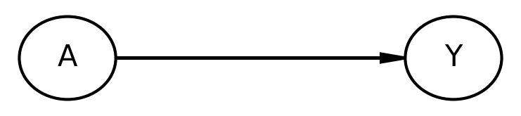
Fig 1. Causal graph showing that A causes Y.
In contrast, if the two outcomes are the same, we say that action A has no causal effect on outcome Y. We can draw that A has no causal effect on Y by making sure there is no arrow between A and Y:
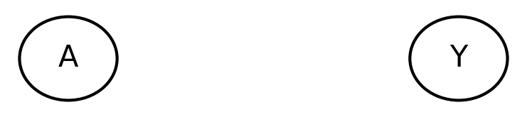
Fig 2. Causal graph showing that A has no causal effect on Y.
What is an "action"? Think of an action as a treatment (intervention) or an exposure. Treatments are things we can experimentally manipulate, like in randomised controlled trials. In contrast, exposures in observational studies can’t be manipulated.
For a single action, there are at least two potential outcomes: outcome Y when action A is taken (

In the causal inference literature, authors refer to outcomes under different actions as potential outcomes because they could happen, or as counterfactuals (counter to the fact) since one or some of those outcomes might not actually happen. We can think of potential outcomes or counterfactuals as "what might happen in a parallel universe?" or "what might happen in a different possible world?".
There is a causal effect for an individual if a person’s potential outcome Y under action a=1 is not equal to the person’s potential outcome Y under action a=0, or 
Average causal effects
What about average causal effects? Can an average causal effect of a group of individuals be identified using data? The short answer is yes, sometimes. Let’s see how to measure an average causal effect if we could see all potential outcomes.
Let’s think about the actions of a group of people. The table below shows our group (persons 1-20), their actions (if they ate leftovers or did not eat leftovers), and their potential outcomes (if they got sick or did not get sick). The data in this table are not realistic because in real life, only one action and its potential outcome can be observed for each person. But let’s use these data to see how average causal effects could be identified using data.
Table 1.1 Actions (ate or not ate leftovers) and potential outcomes (sick or not sick) of a group of 20 people.
| Person | Ate leftovers | Not ate leftovers |
|---|---|---|
| 1 | sick | sick |
| 2 | sick | sick |
| 3 | sick | sick |
| 4 | sick | sick |
| 5 | sick | sick |
| 6 | not sick | sick |
| 7 | not sick | sick |
| 8 | not sick | sick |
| 9 | not sick | sick |
| 10 | not sick | sick |
| 11 | sick | not sick |
| 12 | sick | not sick |
| 13 | sick | not sick |
| 14 | sick | not sick |
| 15 | sick | not sick |
| 16 | not sick | not sick |
| 17 | not sick | not sick |
| 18 | not sick | not sick |
| 19 | not sick | not sick |
| 20 | not sick | not sick |
For action, if all 20 people ate leftovers (middle column), the proportion of those who got sick is 10/20 = 0.5.
For the other action, if all 20 people did not eat leftovers (right column), the proportion of those who got sick is 10/20 = 0.5. Notice, for each action, we calculated the counterfactual outcome just by counting those who got sick (10) divided by the total number of people in the group (20). This is the same as calculating the average counterfactual outcome of the group.
There is an average causal effect for a group of individuals if a group of persons’ average potential outcome Y under action a=1 is not equal to the group of persons’ average potential outcome Y under action a=0. Our food poisoning example has binary outcomes, so we refer to the probability/risk/odds of getting sick. To define an average causal effect more generally so we can include mean differences for continuous outcomes, we say that there is an average causal effect if the expected potential outcome Y under action a=1 is not equal to the expected potential outcome Y under action a=0, or ![E[Y^{a=1}] \neq E[Y^{a=0}]](https://s0.wp.com/latex.php?latex=E%5BY%5E%7Ba%3D1%7D%5D+%5Cneq+E%5BY%5E%7Ba%3D0%7D%5D&bg=ffffff&fg=111111&s=0&c=20201002)
In our example, the proportion of those who got sick after eating leftovers is the same as the proportion of those who got sick even though they did not eat leftovers. So, on average, there is no causal effect of eating leftovers on health for this group of people.
Summary and important points
-
Individual causal effects can’t be identified from data because counterfactual outcomes under different actions are missing.
-
Sometimes, average causal effects can be identified using data even if individual causal effects can’t.
-
The absence of an average causal effect does not imply the absence of an individual causal effect. E.g. person 1 has no individual causal effect of eating leftovers, but person 11 does.
Also note,
-
Causal effects need to be attributed to specific actions. Eating leftovers is a useful example, but it seems too general. What kind of leftovers were eaten? How long was the food leftover for? How much was eaten? Etc.
-
If there are more than 2 actions (e.g. ate leftovers, not ate leftovers, ate something else), the comparison of interest needs to be specified.
In the next post, we will discuss how to measure or quantify causal effects.
Reference
Hernán MA, Robins JM (2020). Causal Inference: What If. Chp 1.1-1.2, 6.1. Boca Raton: Chapman & Hall/CRC.
See also: Table of contents
Python code
'''
Causal graphs for illustration were created using code templates from ported PyMC3 code of:
McElreath R (2020) Statistical Rethinking: A Bayesian course with examples in R and Stan (2nd Ed).
 Florida, USA: Chapman and Hall/CRC, p 316-318.

Code template from Chp 5 notebook at:
https://github.com/pymc-devs/resources/tree/master/Rethinking_2

Recommendations:
1. Run script in virtual environment; `daft` package reconfigures matplotlib settings on import
2. Run separate sections of the script manually in a console to save causal graphs with correct aspect
'''

import matplotlib.pyplot as plt
import daft
from causalgraphicalmodels import CausalGraphicalModel

# Section 1: A -> Y
dg = CausalGraphicalModel(nodes=["A", "Y"], edges=[("A", "Y")])
pgm = daft.PGM()
coordinates = {"A": (0, 0), "Y": (2, 0)}
for node in dg.dag.nodes:
    pgm.add_node(node, node, *coordinates[node])
for edge in dg.dag.edges:
    pgm.add_edge(*edge)
pgm.render()
plt.gca().invert_yaxis()

# Section 2
plt.savefig('fig-1.png', dpi=300)
plt.close()

# Section 3: A   Y
dg = CausalGraphicalModel(nodes=["A", "Y"], edges=[("A", "Y")])
pgm = daft.PGM()
coordinates = {"A": (0, 0), "Y": (2, 0)}
for node in dg.dag.nodes:
    pgm.add_node(node, node, *coordinates[node])
pgm.render()
plt.gca().invert_yaxis()

# Section 4
plt.savefig('fig-2.png', dpi=300)
plt.close()
