Independent t-test as a linear model in R

Posted on June 8, 2017 by Martin Héroux Leave a comment

My last two posts have shown how to perform an independent t-test in the R programming language and the Python programming language. For those of you who are familiar with statistics, you likely know that an independent t-test is equivalent to performing an one-way analysis of variance on the data. What you may not have realised is that both these statistical tests are actually linear models in disguise.

In the present post we will learn a little about linear models and figure out how to perform an independent t-test using a linear model approach. Why bother with this? Linear models can be extended to perform more complex statistical analyses, but they can be confusing to newcomers. A simple example like this one is a good place to start.

The dataset: Environmental impact of pork and beef

In our previous R post, we created a fictional dataset on the environmental impact (measured in kilograms of carbon dioxide) of pork and beef production. The dataset was created using the following R code:

# Number of animals in each group 
n = 30
names=c(rep("pork", n) , rep("beef", n))
# Draw samples from two different populations
value=c(sample(0:500, n, replace=T), sample(100:600, n, replace=T))
# Create a dataframe
data=data.frame(names,value)

When I initially executed these lines of code, it generated the following data:

Figure 1: Grey dots represent each animal in our sample. The means and standard deviations are also plotted.

Random sampling. Because the data is generated using sample(), executing the code a second time will generate a different dataset. This is because we will be using a different sample of values. So don’t worry if your dataset and statistical results are different than mine. The key thing is that you obtain the same results using the t.test() function or the linear model approach.

Linear model basics

All statistical procedures are pretty much the same. They are all versions of the following model:

$outcome_i = (model) + error_i \label{_auto1}$

The structure of a basic linear model is:

$A_i = (b_0 + b_1G_i) + \epsilon_i$

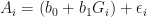
In this equation, Ai represents the dependent variable (i.e., the outcome variable), b0 is the intercept, b1 is the weighting of the independent variable (i.e., predictor) and Gi is the independent variable. The funny looking E, the Greek letter epsilon, represents the error term and is the variance in the data that cannot be explained by our model.

Thinking about our dataset in terms of linear models

The above generic formula is a little cryptic. As a more concrete example, let’s write out the linear model for our sample dataset:

$envImpact_i = (b_0 + b_1animal_i) + \epsilon_i$

when a study has two conditions, beef and pork in our case, the independent variable has only two values. The simplest ways to code these two variables is to assign the value of 0 to one of the groups and 1 to the other. These kind of variables are sometimes referred to as dummy variables. While the assignment of 0 and 1 can be done manually, R recognizes the names variable we created as a factor and automatically assigns these values for us.

R assigned 0 to beef and 1 to pork. So, to determine the environmental impact for beef, we set the independent variable to 0:

$\overline{X}_{beef} = b_0 + (b_1 \times 0)$
$b_0 = \overline{X}_{beef}$
$b_0 = 353.6$

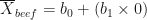
This tells us that the intercept b0 is equal to 353.6. If you look back to the previous R post, the value of the intercept is the same as the mean environmental impact of beef. This is pretty cool, but why is the intercept equal to the mean environmental impact of beef? Below is a marked-up version of our figure, which may help us understand what is going on.

Figure 2: R has assigned beef the dummy variable 0 and pork the dummy variable 1. The intercept of a linear model applied to this data is equal to the mean of the beef data: 353.6. The slope of the line fit to our data is -91.57, which is the difference between the mean value for beef and the mean value for pork. So 353.6 -91.57 = 262.03, which is the mean environmental impact of pork.

What happens when pork is added to our model? Let’s set our independent variable to 1:

$\overline{X}_{pork} = b_0 + (b_1 \times 1)$
$b_1 = \overline{X}_{pork} - \overline{X}_{beef}$
$b_1 = -91.57$

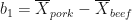
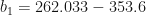
The above equation tells us that b1, the weighting factor of our independent variable is -91.57. Where does this number come from? Again, if you remember the previous R post, the mean environmental impact of pork was 262.0333. Thus, b1 is equal to the mean value of pork minus the mean value of beef, or:

$b_1 = \overline{X}_{pork} - \overline{X}_{beef}$
$b_1 = 262.033 - 353.6$
$b_1 = -91.57$

If you look back to Figure 2, do you notice anything interesting? The slope of the line that was fit to our data is equal to b1, which is also equal to the diffence between the mean pork value and mean beef value. This is pretty cool! Looking at the graph, it is clear that 353.6 – 91.57 is equal to 262.03.

This tells us that when we fit a linear model to our data, the intercept of the line is equal to the mean value of the first independent variable (i.e., beef) and the slope is equal to the difference between the mean value of our first and second independent variables.

Analysing our dataset using a linear model

The final piece of the puzzle is determining whether b1 (i.e., the slope, the difference between beef and pork) is significantly different from zero. To do this we can analyse our dataset using a linear model. Remember that our dataframe data has two columns, names that specifies the names of our independent variable (beef and pork) and value that specifies the values for each of the beef and pork in our sample.

> t.test.lm = lm(value ~ names, data=data) 
> summary(t.test.lm)

Call:
lm(formula = value ~ names, data = data)

Residuals:
    Min      1Q  Median      3Q     Max 
-262.03  -90.96   15.18  124.83  239.40 

Coefficients:
            Estimate   Std. Error  t value   Pr(>|t|)    
(Intercept)   353.60      27.23     12.984
namespork     -91.57      38.51     -2.377   0.0208 *  
---
Signif. codes:  0 *** 0.001 ** 0.01 * 0.05 . 0.1   1

Residual standard error: 149.2 on 58 degrees of freedom
Multiple R-squared:  0.0888,    Adjusted R-squared:  0.07309 
F-statistic: 5.652 on 1 and 58 DF,  p-value: 0.02075

Looking at the Coefficients portion of the summary, we see that the intercept (i.e., b0) is 353.6 and b1 (i.e., namespork) is -91.57. An important piece of information is the t-value and p-value associated with the b1 coefficient. Notice that the t-value and p-value are exactly the same as those we obtained using a traditional t-test in our previous R post.

So now we now that the mean difference between groups is -91.57 and it is statistically significant with t-value = -2.377 and p-value = 0.0208.

The last thing we need to know is the 95% confidence interval associated with the difference between groups. The R output tells us that the standard error association with b1 is 38.51. When dealing with larger samples (i.e., greater than 50 or so), a quick and dirty way to calculate a 95% confidence interval is to compute the margin of error using 1.96 (equivalent to two standard deviations on t-distribution with a very large sample, or a z-distribution). If you are not familiar with 95% confidence intervals and margins of error, this topic was dicussed in the post on running an independent t-test in Python.

For our present example, 38.51 * 1.96 = 75.47. So our 95% confidence interval is [-91.57 – 75.47] to [-91.57 + 75.57], which is -16.1 to -167.05. This confidence interval is close to what we obtained when we ran a traditional t-test. However, it is not exactly the same. The reason is that for a t-distribution for 60 samples, the value corresponding to two standard deviations is slightly larger than 1.96. So, similar to what we did in Python, we can retrieve the correct values using the qt function of the Student t distribution for 58 degrees of freedom (see Python post for further details):

qt(c(.025, .975), df=58)
-2.001717  2.001717

If we multiply our standard error by these new values, we obtain the correct 95% confidence interval: -14.5 to -168.7.

Summary

We learned how to perform an independent t-test using a linear model. While this may seem complicated, it helped introduce some of the key concepts and terminology of linear models. This will prove useful when we learn about more complicated linear models in future posts.

tagged with linear model, R, statistics, t-test

R
Tutorials