In a previous blog, we applied simple linear regression to an interesting problem: how well does a measure of wine density account for alcohol content. This was considered simple linear regression because we had one outcome variable (alcohol content) and one predictor variable (wine density). We can extend this approach to have more than one predictor. Specifically, we can use multiple linear regression to find the linear combination of predictors that correlate maximally with the outcome variable.

In this post we will return to our white wine dataset to learn how to perform a multiple linear regression in R. Please refer to the previous post for a description of the dataset.

Additional predictors to our model

In our previous post we had one predictor: wine density. We will now include two more predictors: total sulfur dioxide and fixed acidity.

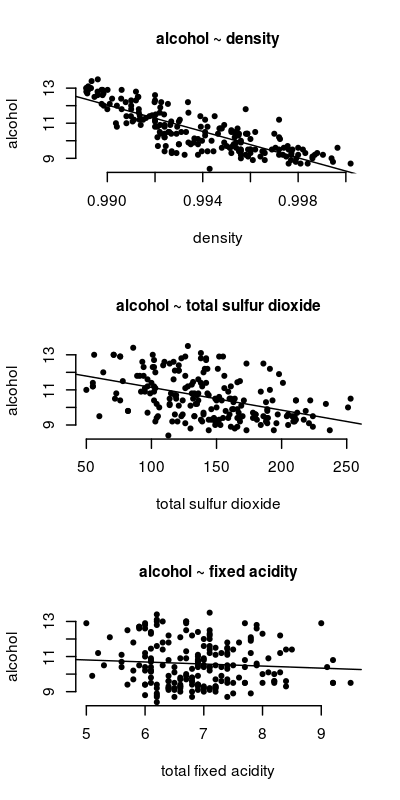
First, let’s look at how each predictor relates to wine alcohol content.

The code to generate the above figure is:

png(file="simple_regression.png",width=400,height=800, res=140)

# Setup for a 3 rows, 1 column figure
par(mfrow=c(3,1))

# Scatterplot of density X alcohol
plot(white$density, white$alcohol,
  xlab="density", ylab="alcohol", main='alcohol ~ density',
  pch=20, cex.main=1, frame.plot=FALSE)

# Calculate simple linear regression model
alc.dens <- lm(alcohol~density, data=white)

# plot regression line
abline(alc.dens)

# Repeat for two other predictors
plot(white$total.sulfur.dioxide, white$alcohol,
  xlab="total sulfur dioxide", ylab="alcohol", main='alcohol ~ total sulfur dioxide',
  pch=20, cex.main=1, frame.plot=FALSE)
alc.sulfDiox <- lm(alcohol~total.sulfur.dioxide, data=white)
abline(alc.sulfDiox)
plot(white$fixed.acidity, white$alcohol,
  xlab="total fixed acidity", ylab="alcohol", main='alcohol ~ fixed acidity',
  pch=20, cex.main=1, frame.plot=FALSE)
alc.acidity <- lm(alcohol~fixed.acidity, data=white)
abline(alc.acidity)

dev.off()

As the figure indicates, wine density is quite related to alcohol content. The relationship is not as strong for total sulfur dioxide, and it is weakest for fixed acidity.

Fitting the multiple linear model

We can now fit a multiple linear model to our data.

The formula for our model is:

Specifically:

Great! Let’s fit our model:

# Set working directory (change to where white.csv is saved)
setwd("~/Desktop")

# Read in the data
white <- read.csv("white.csv", header=TRUE)

# Run multiple linear model
alcohol2 <- lm(alcohol ~ density.thousands + total.sulfur.dioxide + fixed.acidity, data=white)

We can see the results of our model by calling the summary() function on our model object.

summary(alcohol2)

Call:
lm(formula = alcohol ~ density + total.sulfur.dioxide + fixed.acidity, 
    data = white)

Residuals:
     Min       1Q   Median       3Q      Max 
-1.86641 -0.52408  0.08267  0.51176  1.84442 

Coefficients:
                       Estimate Std. Error t value Pr(>|t|)    
(Intercept)           3.992e+02  2.147e+01  18.592  < 2e-16 ***
density              -3.924e+02  2.184e+01 -17.969  < 2e-16 ***
total.sulfur.dioxide  4.268e-04  1.375e-03   0.310  0.75665    
fixed.acidity         1.881e-01  6.241e-02   3.014  0.00292 ** 
---
Signif. codes:  0 ‘***’ 0.001 ‘**’ 0.01 ‘*’ 0.05 ‘.’ 0.1 ‘ ’ 1

Residual standard error: 0.6939 on 196 degrees of freedom
Multiple R-squared:  0.6992,    Adjusted R-squared:  0.6946 
F-statistic: 151.8 on 3 and 196 DF,  p-value: < 2.2e-16

Multiple R-squared. This value tells us how well our model fits the data. In this case it is equal to 0.699. This means that, of the total variability in the simplest model possible (i.e. intercept only model) calculated as the total sum of squares, 69% of it was accounted for by our linear regression model.

F-test and p-value. These values tell us that our multiple linear regression is statistically significant.

Individual predictors. When a model has a single predictor, a significant F-test indicates that the predictor significantly predicts the outcome variable. However, this is not true in multiple regression. Therefore, we have to look at each predictor’s respective t values and p-values (Pr(<|t|).

In the summary output above, R returns coefficients for the intercept of our linear model (sometimes referred to as and our predictor variables (i.e. . We see that the coefficient associated with density and fixed acidity are both statistically significant. Thus, we can re-write our model formula as:

Note that because it was not significant, and because its coefficient is very small, removing total sulfur dioxide from our equation will have little impact on our estimate of alcohol content.

> library(QuantPsyc)
> lm.beta(alcohol2)
     density   total.sulfur.dioxide        fixed.acidity 
 -0.86396550           0.01452874           0.12387068

Summary

In this post we learned how to perform multiple linear models in R. However, it is important to note that this is just the tip of the iceberg.

There are times when we might have many predictor variables and we want to find the subset of these predictors that best predict our dependent variable. Alternatively, we might have a few candidate models and want to determine which model best predicts our outcome variable, which model is the most valid. However, I will leave it to you to read up on these aspects of regression analysis.

In our next post we will learn how to assess our regression models using diagnostic tests.