Statistics you are interested in: simple linear regression – part 3

In the first and second posts of this series, we performed simple linear regression of a continuous outcome on a single continuous predictor, but we also learned it is possible to include binary or categorical predictors in such regression models. How is this be done?
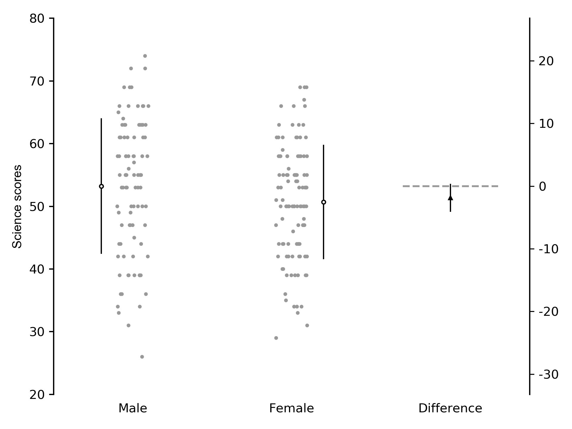
The hsb2.csv dataset we have been using also contains the variable female where male participants are coded 0 and female participants are coded 1. We could perform a linear regression of science scores on sex. The slope of the line shows the change in science scores for a 1 unit increase in sex. In this example, it shows whether female participants scored differently compared to male participants. Because the predictor variable is binary (i.e. male vs. female), performing linear regression of a continuous outcome on a single binary predictor is the same as performing a t-test. We perform the regression and plot the between-group difference and 95% CI. Python code to perform the regression is shown, as well as individual subject data in Figure 1:
import pandas as pd
import matplotlib.pyplot as plt
import statsmodels.formula.api as smf

df = pd.read_csv('hsb2.csv')

# univariate analysis: effect of female
md1 = smf.ols('science ~ female', df)
md1_fit = md1.fit(reml=True)
print(md1_fit.summary())

Out[1]:
                            OLS Regression Results
==============================================================================
Dep. Variable:                science   R-squared:                       0.016
Model:                            OLS   Adj. R-squared:                  0.011
Method:                 Least Squares   F-statistic:                     3.285
Date:                Sat, 19 May 2018   Prob (F-statistic):             0.0714
Time:                        16:41:02   Log-Likelihood:                -740.17
No. Observations:                 200   AIC:                             1484.
Df Residuals:                     198   BIC:                             1491.
Df Model:                           1
Covariance Type:            nonrobust
==============================================================================
                 coef    std err          t      P>|t|      [0.025      0.975]
------------------------------------------------------------------------------
Intercept     53.2308      1.032     51.581      0.000      51.196      55.266
female        -2.5335      1.398     -1.812      0.071      -5.290       0.223
==============================================================================
Omnibus:                        5.395   Durbin-Watson:                   1.772
Prob(Omnibus):                  0.067   Jarque-Bera (JB):                4.349
Skew:                          -0.258   Prob(JB):                        0.114
Kurtosis:                       2.495   Cond. No.                         2.74
==============================================================================
Figure 1: Individual subject data and within-group mean (SD) descriptive statistics, and between-group mean difference (95% CI) inferential statistics of science scores in male and female subjects.

Because males were coded as 0 and females as 1, the Intercept coefficient is the mean science score of male participants, and the slope coefficient is the difference in mean science scores between female and male participants (direction: female – male). The 95% CI of the difference crosses 0, which shows there is no difference between male and female scores: the mean difference between groups is -2.53 points, 95% CI -5.29 to 0.22 points. The width of the confidence interval shows the precision of the estimate of the between-group difference. Loosely speaking, we can say that the between-group difference varies from -5.29 points to 0.22 points, 95% of the time. Confidence intervals are more useful than p values because they show how much the estimate of the between-group difference “jumps around” if the study were repeated many times; that is, the confidence interval allows us to infer the findings in subjects who were not part of the study’s sample.
We might think that some of the variability in science scores is explained by reading scores, so how can we account for this variability? This is done by adding reading scores into the model as a covariate. A covariate is simply another predictor or x variable in a statistical model, and is named because the predictor variables vary together; they co-vary.
In the model below, you will notice that the female predictor is binary, but the read predictor is continuous. Linear regression models can handle continuous and categorical predictors simultaneously (Try doing that with an ANOVA!). We also include some code to write the regression output from both models to the text file results.txt, which is stored in the working directory. Individual subject data and summary statistics are shown in Figure 2:
# multivariate analysis: effect of female adjusted for effect of reading scores
md2 = smf.ols('science ~ female + read', df)
md2_fit = md2.fit(reml=True)
print(md2_fit.summary())

file = 'results.txt'
open(file, 'w').close()
with open(file, 'a') as file:
    file.write('\n--------------------')
    file.write('\nTest between independent groups')
    file.write('\n--------------------')
    file.write('\n')
    file.write('\nEffect of being female on science scores:')
    file.write('\n')
    file.write('\n' + str(md1_fit.summary()))
    file.write('\n')
    file.write('\nEffect of being female on science scores, adjusting for reading scores:')
    file.write('\n')
    file.write('\n' + str(md2_fit.summary()))

Out[2]:
                            OLS Regression Results
==============================================================================
Dep. Variable:                science   R-squared:                       0.406
Model:                            OLS   Adj. R-squared:                  0.400
Method:                 Least Squares   F-statistic:                     67.33
Date:                Sat, 19 May 2018   Prob (F-statistic):           5.21e-23
Time:                        16:57:47   Log-Likelihood:                -689.72
No. Observations:                 200   AIC:                             1385.
Df Residuals:                     197   BIC:                             1395.
Df Model:                           2
Covariance Type:            nonrobust
==============================================================================
                 coef    std err          t      P>|t|      [0.025      0.975]
------------------------------------------------------------------------------
Intercept     21.3422      2.918      7.314      0.000      15.588      27.097
female        -1.8754      1.091     -1.720      0.087      -4.026       0.275
read           0.6037      0.053     11.369      0.000       0.499       0.708
==============================================================================
Omnibus:                        1.134   Durbin-Watson:                   2.030
Prob(Omnibus):                  0.567   Jarque-Bera (JB):                0.846
Skew:                           0.142   Prob(JB):                        0.655
Kurtosis:                       3.143   Cond. No.                         288.
==============================================================================
Figure 2: Individual subject data and within-group mean (SD) descriptive statistics, and between-group mean difference (95% CI) inferential statistics of science scores in male and female subjects, adjusting for reading scores.
We are interested in the coefficients for Intercept and female, not for read because that is simply a control variable. In this example, we see that adjusting for reading scores has narrowed the 95% CI, but the overall conclusion is the same: science scores in males and females are no different, adjusting for reading scores (mean difference -1.88, 95% CI -4.03 to 0.28).
Summary
We performed simple linear regression of a continuous outcome on a binary predictor, with and without covariate adjustment.
Finally, we saved the output from the regression models to a text file.
