We introduced simple linear regression in a previous series and learned how to perform it in R (1, 2). What is the theory behind simple linear regression? How is it used to understand relationships between variables? What is another way to perform it in Python?

The hsb2.csv dataset (available here) contains demographic and academic test scores data from 200 students. We import the data using Python’s Pandas package and print the first few lines to view the variables:

import pandas as pd
import matplotlib.pyplot as plt
import statsmodels.formula.api as smf

df = pd.read_csv('hsb2.csv')
print(df.head())

Out[1]:
    id  female  race  ses  schtyp  prog  read  write  math  science  socst
0   70       0     4    1       1     1    57     52    41       47     57
1  121       1     4    2       1     3    68     59    53       63     61
2   86       0     4    3       1     1    44     33    54       58     31
3  141       0     4    3       1     3    63     44    47       53     56
4  172       0     4    2       1     2    47     52    57       53     61

We are interested in the relationship between reading and science scores. First, we visualise the individual subject data in a scatterplot:

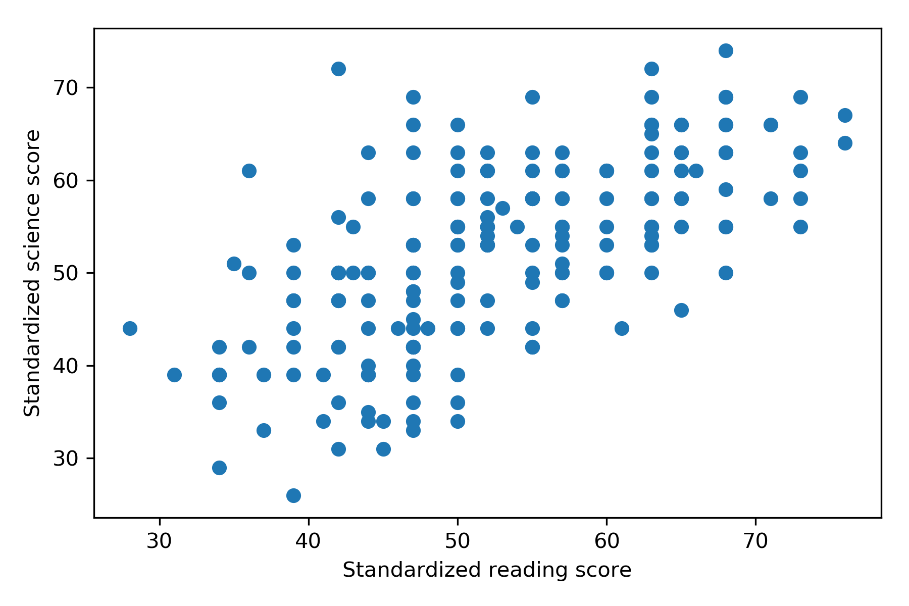
Each data point represents science and reading scores from a single subject. Since one data point provides no information about another data point (i.e. the data are not correlated), we say that the data are statistically independent.

Simple linear regression can be used to determine how the average value of the continuous outcome y varies with the value of a single explanatory variable x (also called a predictor). Here, the outcome is science scores and the explanatory variable is reading scores. Using ordinary least squares estimation, we draw a line of best fit through the data such that the distance of each data point from the line is minimised, and the slope of the line shows how much science scores change for an increase in 1 unit of reading scores.

Using the Statsmodels package, we perform ordinary least squares (OLS) regression of science on reading scores and plot the line of best fit:

md = smf.ols('science ~ read', df)
md_fit = md.fit(reml=True)

intercept = md_fit.params[0]
slope = md_fit.params[1]

fig, ax = plt.subplots(figsize=(6,4))
ax = plt.scatter(df.read, df.science)
plt.xlabel('Standardized reading score')
plt.ylabel('Standardized science score')
xstart, xstop = min(df.read), max(df.read)
ystart, ystop = xstart * slope + intercept, xstop * slope + intercept
plt.plot([xstart, xstop], [ystart, ystop], 'r-')
fig.tight_layout()
plt.savefig('regress.png', dpi=300)

The continuous regression line captures the overall trend that science scores increase as reading scores increase, however it is clear that for any given reading score, there is a lot of variability in science scores. This variability could be due to measurement error, variability between students, and other unmeasured variables that determine science scores.

Using this estimation procedure says:

Science score = Intercept + (Slope x Reading score) + error

The statistical assumptions of this regression model are concerned with how the errors of the outcome (i.e. the last term in the equation) are distributed. Specifically, the model assumes the errors are statistically independent, Normally distributed, and have constant variance at every reading score. Violations of the assumption of Normality and constant variance are in general not too bad, but violation of the assumption of independence is bad.

In contrast, no assumptions about distribution of the predictor are made. It is possible to include predictors that are binary, categorical or discrete (e.g. counts) in such models.

In the next post, we will print the output from the OLS regression and learn how to interpret it.

Summary

We performed simple linear regression of a continuous dependent outcome on a single continuous explanatory variable using ordinary least squares estimation in Python’s Statsmodels package.

We viewed a scatterplot of individual subject data and fitted a straight line of best fit through the data.

Reference

Vittinghoff E, Glidden DV, Shiboski SC, McCulloch CE (2010) Regression methods in biostatistics. Linear, logistic, survival and repeated measures models. Springer, New York.