Python: Analysing EMG signals – Part 2

Posted on August 16, 2016 by Joanna Diong 5 comments

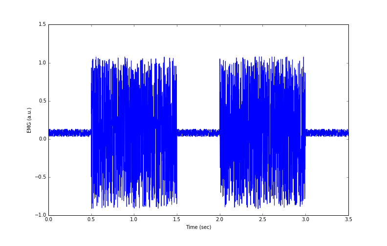
In the previous lesson, we simulated data of two EMG ‘bursts’ during a muscle contraction. The data are shown in Figure 1.

Figure 1: Simulated EMG data from 2 muscle contractions

The code to generate Figure 1 and the explanations are as follows:

import numpy as np
import matplotlib.pyplot as plt
%matplotlib inline

# simulate EMG signal
burst1 = np.random.uniform(-1, 1, size=1000) + 0.08
burst2 = np.random.uniform(-1, 1, size=1000) + 0.08
quiet = np.random.uniform(-0.05, 0.05, size=500) + 0.08
emg = np.concatenate([quiet, burst1, quiet, burst2, quiet])
time = np.array([i/1000 for i in range(0, len(emg), 1)]) # sampling rate 1000 Hz

# plot EMG signal
fig = plt.figure()
plt.plot(time, emg)
plt.xlabel('Time (sec)')
plt.ylabel('EMG (a.u.)')
fig_name = 'fig2.png'
fig.set_size_inches(w=11,h=7)
fig.savefig(fig_name)

Lines 1-3. Import libraries. Use %matplotlib inline if working in an IPython or Jupyter notebook, or in a qtconsole (QuickTime toolkit console).

Lines 6-7. Get 1000 random samples from a uniform distribution of values between -1 and 1. (In a uniform probability distribution, any value within the interval specified has equal probability of being drawn.) To each of these values, add an offset value of 0.08. Perform these procedures to generate EMG data of muscle contractions burst1 and burst2.

Line 8. To generate EMG data for resting muscle in quiet, get 500 random samples from a uniform distribution of values between -0.05 and 0.05. To each value, add an offset of 0.08.

Line 9. Join (concatenate) the simulated EMG data for quiet and burst periods, and assign these values to the variable emg.

Line 10. Create a time variable to indicate that EMG data were sampled at 1000 Hz (ie. 1000 times per second): using a for loop within a list comprehension, generate a list of integer values ranging from 0 to the length of the variable emg, increasing by steps of 1. Take each value in the list and divide it by 1000. Then convert the list of values into a numpy array.

Lines 13-19. Create a figure object called fig so we can refer to the whole figure later. Plot time and emg data, label the x and y axes. Name the figure, set its size and save it.

List comprehensions. Python has a neat syntax functionality called list comprehensions to create a list in one line of code. To write a list comprehension, write an expression and a for loop within square brackets [ ]. In the example above, the expression is i/1000. The list comprehension here is equivalent to:
1
    2
    3
    4
    5
time = []
    for i in range(0, len(emg), 1):
        i = i/1000
        time.append(i)
    np.array(time)

What are some of the problems with our simulated EMG signal?

Baseline EMG values have an offset from zero. This could be due to experimental limitations. An offset in the baseline means that EMG values during contraction also have an offset.
Baseline EMG values are noisy. That is, even when muscles were relaxed, we could not experimentally prevent nonsense signals from being recorded.
The EMG potential difference swings from negative to positive values. This means if we wanted to calculate an average or mean EMG at present, the negative and positive values will cancel out!

In the next lesson we will discuss how some of these problems can be solved using techniques to process EMG data.

Reference

Konrad P (2006) The ABC of EMG – A practical introduction to kinesiological electromyography. Noraxon USA Inc.

Posts in series

tagged with EMG, Python, signal analysis

5 comments

Al3Co

January 22, 2017 11:11 am

Hi Joanna, yep, you are right, now everything its clear now your code works perfect, was the python version, I didn’t check that.

Thanks.

from __future__ import division #only for Python 2.7
import numpy as np
import matplotlib.pyplot as plt # matplotlib inline
import time
figureName = time.strftime("%Y%m%d-%H%M%S") #File name

# simulate EMG signal
burst1 = np.random.uniform(-1, 1, size=1000) + 0.08
burst2 = np.random.uniform(-1, 1, size=1000) + 0.08
quiet = np.random.uniform(-0.05, 0.05, size=500) + 0.08
emg = np.concatenate([quiet, burst1, quiet, burst2, quiet])
time = np.array([i/1000.0 for i in range(0, len(emg), 1)]) # sampling rate 1000 Hz

# plot EMG signal
fig = plt.figure()
plt.plot(time, emg)
plt.xlabel('Time (mili-sec)')
plt.ylabel('EMG (a.u.)')
fig_name = figureName + '.png'
fig.set_size_inches((11, 7))
fig.savefig(fig_name)
print 'output file name: ', fig_name

LikeLike

Aldo
January 20, 2017 9:25 am

#Hey there,
#I ran your code and it has little mistakes, please review again, this (below) is a little modification jumping the “time” variable.
#Regards

import numpy as np
import matplotlib.pyplot as plt
#matplotlib inline
import time
figureName = time.strftime(“%Y%m%d-%H%M%S”)
w = 11
h = 7

simulate EMG signal

burst1 = np.random.uniform(-1, 1, size=1000) + 0.08
burst2 = np.random.uniform(-1, 1, size=1000) + 0.08
quiet = np.random.uniform(-0.05, 0.05, size=500) + 0.08
emg = np.concatenate([quiet, burst1, quiet, burst2, quiet])
time = np.array([i/1000 for i in range(0, len(emg), 1)]) # sampling rate 1000 Hz

#print ‘b1: ‘, burst1, ‘b2: ‘, burst2, ‘quiet: ‘, quiet, ’emg: ‘, emg, ‘time: ‘, time
print ‘Length time : ‘, len(time)
print ‘Length emg : ‘, len(emg)

plot EMG signal

fig = plt.figure()
#plt.plot(time, emg)
plt.plot(emg)
plt.xlabel(‘Time (mili-sec)’)
plt.ylabel(‘EMG (a.u.)’)
fig_name = figureName + ‘.png’
fig.set_size_inches((w, h))
fig.savefig(fig_name)
print ‘output file name:’, fig_name

LikeLike

Reply
- Joanna Diong
  January 20, 2017 11:02 am
  
  Hi Aldo, thanks for this but you will need to give more specific details on where you think the little mistakes are: apart from the time variable change, which line in your code was different from the one in the post?
  
  On running your code, I noticed in line 28 of your code: plt.plot(emg) you chose to plot only the EMG values whereas in line 14 of the code in the post: plt.plot(time, emg) I plotted EMG values on the time variable I built. Doing it your way plots the EMG values by their sample number, so it makes the x-axis look like it is plotted in milliseconds rather than seconds, but the x-axis unit is actually sample number. This is the only key difference I could find.
  
  LikeLike
  
  Reply
  - Al3Co
    January 21, 2017 1:43 pm
    
    Hello Joanna, please copy-paste and run your code written here in this post, you will see that your code does not generate the “Figure 1” as you mention, I have ran it on Linux, Mac and Windows and always got the same result (don’t the figure that you are mentioning). There is not other relevant difference than that line <plt.plot(emg)>. If you want to I can send you by email the Figures that your code is generating.
    
    LikeLike
  - Joanna Diong
    January 21, 2017 10:40 pm
    
    Hi Aldo, that was very interesting. I developed the code in Python 3 but I think you are running it in Python 2 (judging from the way your print statements were written). If so, when you create the time variable in line 10 of the code, Python 2 performs floor division and rounds the floating point numbers to integers. To fix this, specify that the division has to occur with a floating point number:
    time = np.array([i/1000.0 for i in range(0, len(emg), 1)])
    
    Alternatively, to set Python 2 to perform division the way Python 3 does for all instances, write this line at the top of your code:
    from __future__ import division
    
    LikeLiked by 1 person