In the previous lesson we learned that our EMG signal had some problems:

1. Baseline EMG values have an offset from zero.
2. Baseline EMG values are noisy.

Also, the EMG signal possess both negative and positive values. This means if we wanted to calculate an average or mean EMG, the negative and positive values will cancel out.

We can apply 3 processing address these issues with the EMG signal. Specifically, we will (1) remove the mean value from the signal, (2) filter the signal and (3) rectify the signal. I will demonstrate how each technique changes the EMG signal. Key or new bits of code will be annotated in text below the code sections. Graphing code is long but repetitive; you will get the hang of it after awhile.

(1) Remove mean EMG

 1
 2
 3
 4
 5
 6
 7
 8
 9
10
11
12
13
14
15
16
17
18
19
20
21
22
23
24
25
26
27
28
29
30

# if using IPython: check variables from previous lesson are still in workspace
%whos

# process EMG signal: remove mean
emg_correctmean = emg - np.mean(emg)

# plot comparison of EMG with offset vs mean-corrected values
fig = plt.figure()
plt.subplot(1, 2, 1)
plt.subplot(1, 2, 1).set_title('Mean offset present')
plt.plot(time, emg)
plt.locator_params(axis='x', nbins=4)
plt.locator_params(axis='y', nbins=4)
plt.ylim(-1.5, 1.5)
plt.xlabel('Time (sec)')
plt.ylabel('EMG (a.u.)')

plt.subplot(1, 2, 2)
plt.subplot(1, 2, 2).set_title('Mean-corrected values')
plt.plot(time, emg_correctmean)
plt.locator_params(axis='x', nbins=4)
plt.locator_params(axis='y', nbins=4)
plt.ylim(-1.5, 1.5)
plt.xlabel('Time (sec)')
plt.ylabel('EMG (a.u.)')

fig.tight_layout()
fig_name = 'fig2.png'
fig.set_size_inches(w=11,h=7)
fig.savefig(fig_name)

Line 2. Use this IPython magic command to check required variables from the previous session are still in the workspace. Objects for numpy and matplotlib libraries should be present.

Line 5. Calculate the mean (average) of the whole signal and remove it from the signal.

We observe in Figure 1 that removing the mean value brings the whole signal down so the average now sits at 0 volts.

Figure 1: Offset vs mean-corrected EMG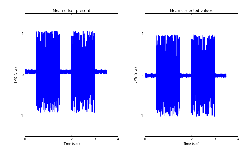

(2) Filter EMG signal

 1
 2
 3
 4
 5
 6
 7
 8
 9
10
11
12
13
14
15
16
17
18
19
20
21
22
23
24
25
26
27
28
29
30
31
32
33
34
35

import scipy as sp
from scipy import signal

# create bandpass filter for EMG
high = 20/(1000/2)
low = 450/(1000/2)
b, a = sp.signal.butter(4, [high,low], btype='bandpass')

# process EMG signal: filter EMG
emg_filtered = sp.signal.filtfilt(b, a, emg_correctmean)

# plot comparison of unfiltered vs filtered mean-corrected EMG
fig = plt.figure()
plt.subplot(1, 2, 1)
plt.subplot(1, 2, 1).set_title('Unfiltered EMG')
plt.plot(time, emg_correctmean)
plt.locator_params(axis='x', nbins=4)
plt.locator_params(axis='y', nbins=4)
plt.ylim(-1.5, 1.5)
plt.xlabel('Time (sec)')
plt.ylabel('EMG (a.u.)')

plt.subplot(1, 2, 2)
plt.subplot(1, 2, 2).set_title('Filtered EMG')
plt.plot(time, emg_filtered)
plt.locator_params(axis='x', nbins=4)
plt.locator_params(axis='y', nbins=4)
plt.ylim(-1.5, 1.5)
plt.xlabel('Time (sec)')
plt.ylabel('EMG (a.u.)')

fig.tight_layout()
fig_name = 'fig3.png'
fig.set_size_inches(w=11,h=7)
fig.savefig(fig_name)

Line 5-6. Create high and low pass filter settings. A ‘high pass’ filter lets frequencies above that cut-off value pass through, while a ‘low pass’ filter lets frequencies below that cut-off value pass through. Raw surface EMG typically has a frequency content of between 6-500 Hz, with the greatest spectral power between 20-150 Hz. Slow oscillations in the EMG signal are likely due to movement artefacts and fast oscillations are often due to unwanted electrical noise. We can apply a digital filter to let high frequency values above 20 Hz pass through (ie. high pass) and let values below 450 Hz pass through (low pass). The sp.signal.butter command requires values between 0 and 1, so filter frequencies are normalised to the Nyquist frequency, which is half of the sampling rate (note: the sampling rate is sometimes called the Nyquist rate, not to be confused with the Nyquist frequency).

EMG signals should always be recorded with analog band-pass filters, often with similar cut-off frequencies (20-450Hz). Between the analog and digital filters, the analog filter is the important one because it acts as an anti-aliasing filter. This means the filter prevents aliasing (distortion) by a higher frequency, non-EMG signal from being recorded. If an EMG signal is aliased and sampled by the analog-to-digital converter, there is no way get rid of this unwanted noise from the signal. Once the EMG signal is analog bandpass filtered and acquired, many researchers choose to not digitally bandpass filter the EMG signal again in Python or Matlab.

Line 7. Create filter. The scipy butter function is used to design an Nth order Butterworth filter and return the filter coefficients in (B,A) form. So, we specify we want to create a 4th order bandpass filter ([high, low], btype='bandpass'). The order of a filter refers to how well the filter includes wanted frequencies and excludes unwanted frequencies. 4th order Butterworth filters are quite common; the filter order relates to how well the filter attenuates unwanted frequencies outside the selected cut-off frequency. In this line, we create the filter and store filter coefficients in variables b and a.

Line 10. Filter the EMG signal to smooth it. The scipy filtfilt function is used to apply a linear filter to the signal one time forward, one time backwards. Applying a filter to a signal causes a frequency-dependent phase shift. While this phase shift is unavoidable when applying an analog (ie. hardware) filter, the phase shift can be corrected by applying the digital filter backwards. Note that using filtfilt means an 8th order filter is being applied with a slightly narrower frequency bandwidth to what was specified in butter. In this line, we filter the emg_correctmean signal.

Figure 2 shows the unfiltered EMG signal, and the filtered EMG signal with high frequency values removed.
It is important to understand how changing filter cut-off frequencies changes the properties of the signal, but understandably, it’s hard to see in detail here how removing high frequency values has changed the signal. I will try to demonstrate these changes in the next post. For now, we will leave the cut-off frequencies as is.

Note. One limitation of using simulated signals to demonstrate EMG is that the simulated EMG signal here has an instantaneous onset and offset, which is not physiological. This results in a ringing artifact at the start and end of the simulated EMG signals. This kind of artifact can be seen when harsh filters are applied to evoked potentials (eg. H-reflex, TMS motor evoked potentials) because they rise very sharply. Here however, an instantaneous EMG start is an artefact.

 Figure 2: Unfiltered vs filtered EMG

(3) Rectify EMG signal

 1
 2
 3
 4
 5
 6
 7
 8
 9
10
11
12
13
14
15
16
17
18
19
20
21
22
23
24
25
26
27

# process EMG signal: rectify
emg_rectified = abs(emg_filtered)

# plot comparison of unrectified vs rectified EMG
fig = plt.figure()
plt.subplot(1, 2, 1)
plt.subplot(1, 2, 1).set_title('Unrectified EMG')
plt.plot(time, emg_filtered)
plt.locator_params(axis='x', nbins=4)
plt.locator_params(axis='y', nbins=4)
plt.ylim(-1.5, 1.5)
plt.xlabel('Time (sec)')
plt.ylabel('EMG (a.u.)')

plt.subplot(1, 2, 2)
plt.subplot(1, 2, 2).set_title('Rectified EMG')
plt.plot(time, emg_rectified)
plt.locator_params(axis='x', nbins=4)
plt.locator_params(axis='y', nbins=4)
plt.ylim(-1.5, 1.5)
plt.xlabel('Time (sec)')
plt.ylabel('EMG (a.u.)')

fig.tight_layout()
fig_name = 'fig4.png'
fig.set_size_inches(w=11,h=7)
fig.savefig(fig_name)

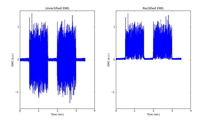
Line 2. Take the absolute of all EMG values (ie. all negative values become positive) so that positive and negative values don’t cancel out when mean EMG is calculated. There is controversy in the EMG analysis field regarding whether EMG signals should be rectified for certain types of analyses (eg. coherence analysis). Another preferred EMG analysis technique is to calculate the root-mean-square (RMS) of the unrectified signal. So, EMG signal rectification may or may not be needed depending on how the signal needs to be analysed.

We observe in Figure 3 that our EMG is entirely positive.

 Figure 3: Unrectified vs rectified EMG

Summary

We can process raw EMG signals by (1) removing the mean EMG value from the raw EMG signal, (2) creating and applying a filter to the EMG signal and (3) rectifying the signal by taking the mathematical absolute of all values. In the next and final post for this series, we will see how changing filter cut-off frequencies changes the filtered signal.