In the previous post we plotted repeated measures data from 10 subjects under 2 conditions. There are different ways to analyse small datasets. We could apply parametric methods to analyse the data values, such as describing the data with means and standard deviations, and calculating a paired difference. Or, we could also apply non-parametric methods by analysing data values based on their rank rather than the numeric value. For example, we could calculate the middle (median) value of the data and the range between the 25-75% value (interquartile range), and show these values on a boxplot with the raw data.

 1
 2
 3
 4
 5
 6
 7
 8
 9
10
11
12
13
14
15
16
17
18
19
20
21
22
23
24
25
26
27
28

# plot scatterplot and boxplots of hours of sleep
set.seed(10) # keeps noise in jitter constant
fig <- ggplot(df, aes(x=group, y=extra)) +
  geom_boxplot(width=0.4) +
  geom_point(aes(color=ID), size=5, position=position_jitter(width=0.05)) +
  # Remove comment from line below to plot lines linking points from the same subject for drugs 1 and 2
  # geom_line(aes(x=group, y=extra, group=ID), size=1, alpha=0.5) + 
  xlab('Drug') + 
  ylab('Extra sleep (hour)') +
  theme_bw() + 
  theme(axis.line = element_line(colour="black"),
        panel.border = element_rect(colour="black", size=1),
        panel.grid.major = element_blank(),
        panel.grid.minor = element_blank(),
        panel.background = element_blank(),
        text = element_text(size=18))
print(fig)
# save figure
png(filename="boxplot.png", width=11, height=7, units='in', res=300)
plot(fig)
dev.off()

# reshape dataframe from long to wide format
df_wide <- reshape(df, idvar='ID', timevar='group', direction='wide')
print(df_wide)

# calculate median and IQR of hours of sleep
lapply(df_wide[, 2:3], quantile)

Line 1-21. Code for the boxplot and scatterplot here is nearly identical to graph code previously. At present, the graph is being plotted with data in long format.

Line 23-28. Reshape the data so it is now in wide format ie. repeated observations for each subject are written on the same row, so that each subject has data only over 1 row. Then, calculate the median and IQR values of the outcome (hours of sleep) for each of the conditions (drug 1 and 2) using a list apply function (lapply).

The code generates the following Figure 1:

Figure 1:

 

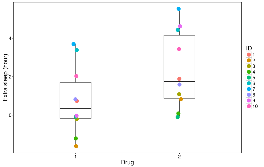
and the following median and IQR of hours of sleep:

1
2
3
4
5
6
7
8

> lapply(df_wide[, 2:3], quantile)
$extra.1
    0%    25%    50%    75%   100% 
-1.600 -0.175  0.350  1.700  3.700 

$extra.2
    0%    25%    50%    75%   100% 
-0.100  0.875  1.750  4.150  5.500 

From the figure, it might be reasonable to think there is a between-condition difference in the medians, but there is also a lot of overlap in the data: this is obvious from the raw data and the interquartile ranges. How can we test whether this difference in the medians is real, and get a measure of precision of this effect? In the next post we will calculate the between-condition difference of the medians and use a resampling technique called bootstrapping to calculate precision about our estimate of the difference of the medians.

Summary

For this small dataset, we calculated the non-parametric median and interquartile range of data in each condition, and plotted these values as boxplots overlaid with raw data points. Next, we will calculate the between-condition difference of the medians and calculate precision about our estimate of the difference of the medians.