Badly behaved data, part 2: Log-transforming values from one sample

Posted on May 4, 2021 by Joanna Diong Leave a comment

To analyse data, researchers often use statistical tests that assume data are Normally distributed in order to apply parameters (mean, SD) of a Normal distribution. These are known as parametric tests. But the assumption that data are Normally distributed does not always hold, so using parametric tests is not the best approach. How can we know if data are Normally distributed?

The best way to determine how data are distributed is to plot and visually inspect the spread of data over the range of values. This is better than using statistical tests of Normality, because these tests do not hold under all conditions and can increase false positive findings.

Describing skewed data

In our previous post, we generated non-Normal data and data with outliers, and visualised these data in plots. Suppose we want to summarise the data on days to discharge from hospital, but these data are skewed. What is a good approach?

We could summarise the data using non-parametric statistics, such as the median and interquartile range (IQR). These statistics analyse the ranks of the data, not the actual data values, and so they do not require the data to have parameters. If we apply a non-parametric procedure here, we rank all days to discharge values from smallest to largest. From all the ranks, report the middle ranked value (median; 50th percentile) and the ranked values over a range (IQR; 25th and 75th percentiles). This is a valid approach to summarising skewed data.

Another approach is to transform the data by taking the logarithm, square root, inverse, or some other function of the data (Bland and Altman 1996). We want a function that allows us to easily interpret the mean and confidence interval (CI). The best transformation for this is the logarithm.

Let’s do the following:

Draw 100 random values of days to discharge from hospital from a log-Normal distribution.
Log-transform the days to discharge data and store this as a new variable.
Plot histograms of days and log(days).
Get summary statistics of days and log(days). Save these to CSV.
Print the means and 95% CI for days, log(days), and anti-logged log(days).

The Python code to execute these steps is shown at the end of this post. Running the code generates this figure:

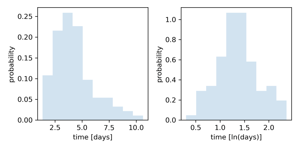
Fig 1. Histogram of time in days show data are skewed with a long tail to the right (left). When days are log-transformed, the histogram shows data are more Normally distributed (right).

As before, simulated days to discharge are right-skewed. But now, the histogram of log-transformed days shows these data are more Normally distributed. Why does a log-transform do this?

How log-transforms work

Generally speaking, log-transforming natural values produces the orders of magnitude of those values. Conversely, back-transforming those orders of magnitude by taking the anti-log returns the natural values (McElreath 2020).

This makes more sense when we think of numbers ranging from very small to very large. For example, using log base 10, an order of magnitude 1 corresponds to a multiple by factor 10. We can relate orders of magnitude to their corresponding logarithms:

Order of magnitude      Corresponds to log10 of
1                       10
2                       100
3                       1000

So on the log scale, someone who is 100 years old is roughly twice as old as a toddler. The log scale compresses large differences between natural values. Which is how it makes skewed data more Normally distributed. Conversely, when we have compressed logged values, we have to explode them (by exponentiating the logged values) to back-transform them into natural values.

All log-transforms require a base. Common bases are $log_{10}$ , $log_{2}$ , or $log_{e}$ (Euler’s number for natural logs, which is $\approx2.71828$ ). You can log-transform using any base, but use the same base for all subsequent calculations. Python’s np.log() performs the natural log transform $log_{e}$ , also written as $ln$ . (I say this as "lonn" which is what I was taught under British-based GCSE math, and also what the Canadians seem to prefer. But apparently the Americans say both syllables "ell enn" or say "natural log" in full. Who’s right? The jury is still out!)

Describing the data

Back to our data. The problem with describing skewed days to discharge using mean and SD parameters is that the mean gets pulled to the right because of the long right tail. However we transformed these data using $log_{e}$ . Since log(days) is now Normally distributed, we can appropriately describe these data using mean and SD. Pulling summary statistics using Pandas describe() produces this report:

             days      lndays
count  100.000000  100.000000
mean     4.271011    1.368203
std      1.828536    0.409152
min      1.352032    0.301609
25%      2.968228    1.087929
50%      3.901672    1.361353
75%      5.061932    1.621746
max     10.627387    2.363434

The mean (SD) of log(days) is 1.36 (0.41) log(days). Good. But what is an average time to discharge of "1.36 log(days)"? No one really thinks in units of log(days). Remember, this is the order of magnitude of days to discharge of factor $e$ , not actual days. We would much prefer a transformation that allows us to interpret the data meaningfully in days.

We could calculate the anti-log of the mean days to discharge as $e^{1.36}$ , since our data were transformed using natural log. Doing so, we get $e^{1.36} = 3.93$ days. Notice that this value is smaller than the mean days to discharge (4.27 days): this is correct. In our example, the anti-logged mean should be smaller than the mean of skewed natural values because it is less biased by the long right tail.

Calculating the anti-log of the standard deviation is more problematic. A standard deviation is calculated using the difference of each value from the mean. But the difference between the log of two numbers is the log of their ratio (see Properties of natural logs, rule 4. Since a ratio is unitless number, it is not possible to back-transform the SD from the log scale to obtain the SD in natural units (days).

The better approach is to calculate the mean and 95% CI on the log scale, then anti-log these values to obtain values in natural units. Below I show the mean (95% CI) for days, log(days) and exponentiated log(days):

Days: 
Mean  4.27, 95% CI  3.91 to  4.63
Ln(days): 
Mean  1.37, 95% CI  1.29 to  1.45
Exp^(Ln(days)): 
Mean  3.93, 95% CI  3.62 to  4.26

Summary

We simulated skewed data, and log-transformed the data to make it more Normally distributed. We visualised natural and transformed data using histograms. Log transforms compress large differences between values in natural units.

The mean from the log scale can be back-transformed (anti-logged) to obtain the mean in natural units, but the SD from the log scale can’t be back-transformed to obtain the SD in natural units. Instead, back-transform the mean (95% CI) from the log scale to obtain the mean (95% CI) in natural units.

References

Bland JM and Altman DG (1996) Statistics notes: Transforming data. BMJ 312: 770.

Bland JM and Altman DG (1996) Statistics notes: Transformations, means, and confidence intervals. BMJ 312: 1079.

McElreath R (2020) Statistical Rethinking: A Bayesian course with examples in R and Stan. (2nd Ed) Florida, USA: Chapman and Hall/CRC, p 94.

Posts in series

Python code

import numpy as np
import matplotlib.pyplot as plt
from scipy.stats import norm, lognorm
import pandas as pd
import statsmodels.stats.api as sms

np.random.seed(15)

# generate days to discharge data
shape = 0.4
scale = 4
days = lognorm.rvs(s=shape, scale=scale, size=100)
days = [day for day in days if day &gt; 0]

# log-transform days to discharge
lndays = np.log(days)

# plot
fig = plt.subplots(figsize=(6, 3))
ax1 = plt.subplot(1, 2, 1)
ax1.hist(days, density=True, histtype='stepfilled', alpha=0.2)
ax1.set_xlabel('time [days]')
ax1.set_ylabel('probability')

ax2 = plt.subplot(1, 2, 2)
ax2.hist(lndays, density=True, histtype='stepfilled', alpha=0.2)
ax2.set_xlabel('time [ln(days)]')
ax2.set_ylabel('probability')

plt.tight_layout()
plt.savefig('figure.png', dpi=300)
plt.close()

# save summary data to CSV
df = pd.DataFrame({'days': days, 'lndays': lndays})
df.describe().to_csv('summary.csv')
print(df.describe())

# print mean (95% CI) of raw and log-transformed data, and the anti-logged values
print(f'\nDays: \nMean {np.mean(days): .2f}, '
      f'95% CI {sms.DescrStatsW(days).tconfint_mean()[0]: .2f} '
      f'to {sms.DescrStatsW(days).tconfint_mean()[1]: .2f}')
print(f'Ln(days): \nMean {np.mean(lndays): .2f}, '
      f'95% CI {sms.DescrStatsW(lndays).tconfint_mean()[0]: .2f} '
      f'to {sms.DescrStatsW(lndays).tconfint_mean()[1]: .2f}')
print(f'Exp^(Ln(days)): \nMean {np.exp(np.mean(lndays)): .2f}, '
      f'95% CI {np.exp(sms.DescrStatsW(lndays).tconfint_mean()[0]): .2f} '
      f'to {np.exp(sms.DescrStatsW(lndays).tconfint_mean()[1]): .2f}')

tagged with log-Normal, logarithm

Research tools and methods