Suppose we want to compare the means of two groups where data are skewed. In the last post, we saw that the mean and 95% CI are preferred to summarise log-transformed data for one sample. Can we use a similar approach to compare means from two log-transformed samples? Well, sort of. It is a little more complicated. Let’s see why.

Let’s simulate data from a randomised controlled trial where days to discharge from hospital (the outcome) were measured in control and treated groups. We know that data on days to discharge are skewed:

1. For control and treated groups, draw 100 random values of days to discharge from log-Normal distributions with identical locations (loc=0) but with different shapes.
2. Log-transform the days to discharge data.
3. Plot histograms of days and log(days).
4. Perform simple linear regression comparing log(days) between both groups.
5. Report the estimates in logged and back-transformed natural values.

The Python code to execute these steps is shown at the end of this post. Running the code generates this figure:

Fig 1. Histograms of time in days (top row) and time in log-days (bottom row) for control (left column) and treated (right column) groups.

Histograms show that days to discharge become more Normally distributed after values are log-transformed. This is good.

Let’s place the data in a Pandas dataframe for further analysis and use long format: vertically stack days and log(days) values from the control and treated groups, and create the column treated where 0 indicates the control group and 1 indicates the treated group. The 0’s and 1’s in treated are dummy codes; the numbers simply indicate the group that each outcome belongs to, but don’t mean anything physiologically. However, assigning 0’s or 1’s to outcomes this way allows us to analyse the data meaningfully later on.

On summarising the values in each group, the treated group mean in days seems smaller than the control group mean (not surprising, since data are skewed) but group means of log(days) are almost identical. This is expected because data were drawn from distributions with identical locations (step 1 of data simulation):

Control group:
        treated        days      lndays
count    100.0  100.000000  100.000000
mean       0.0    5.387911    1.350112
std        0.0    4.969176    0.818304
min        0.0    0.456998   -0.783077
25%        0.0    2.202751    0.789564
50%        0.0    3.806154    1.336412
75%        0.0    6.405810    1.857199
max        0.0   28.235337    3.340574

Treated group:
        treated        days      lndays
count    100.0  100.000000  100.000000
mean       1.0    4.243813    1.364461
std        0.0    1.756280    0.409575
min        1.0    0.999790   -0.000210
25%        1.0    3.013148    1.102982
50%        1.0    3.781147    1.330018

That is, we should expect to find no difference between groups when comparing the means of log(days).

Let’s use simple linear regression (i.e. ordinary least squares, OLS) to compare the means between treated and control groups. Since no other variables are in the model, this is equivalent to an independent t-test. The advantage of doing a regression is that the regression output reports the magnitude of the between-group difference and its precision, the 95% CI. Not just the p value. Reporting how large an effect is and how precisely it was estimated is always more informative than a p value.

We run the simple linear regression using Python’s statsmodels.formula.api. This function allows us to specify a regression model similarly to how models are specified in the R programming language. Summarising the model produces:

                            OLS Regression Results                            
==============================================================================
Dep. Variable:                 lndays   R-squared:                       0.000
Model:                            OLS   Adj. R-squared:                 -0.005
Method:                 Least Squares   F-statistic:                   0.02459
Date:                Thu, 25 Feb 2021   Prob (F-statistic):              0.876
Time:                        20:35:26   Log-Likelihood:                -195.72
No. Observations:                 200   AIC:                             395.4
Df Residuals:                     198   BIC:                             402.0
Df Model:                           1                                         
Covariance Type:            nonrobust                                         
==============================================================================
                 coef    std err          t      P>|t|      [0.025      0.975]
------------------------------------------------------------------------------
Intercept      1.3501      0.065     20.865      0.000       1.223       1.478
treated        0.0143      0.092      0.157      0.876      -0.166       0.195
==============================================================================
Omnibus:                        4.417   Durbin-Watson:                   1.891
Prob(Omnibus):                  0.110   Jarque-Bera (JB):                5.657
Skew:                           0.071   Prob(JB):                       0.0591
Kurtosis:                       3.812   Cond. No.                         2.62
==============================================================================

Visually, what the model does is this:

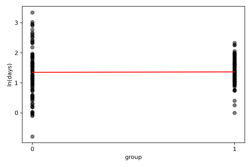
Fig 2. Individual participant data of log(days) data in control (coded 0) and treated (coded 1) groups. The straight line from the simple linear regression passes through the means of both groups (red line).

Interpreting regression output

The key pieces of information from the Statsmodels output are reported at the lines Intercept and treated. The intercept of a line is where it cuts the vertical axis. The slope of a line indicates how much it rises or falls as the value on the horizontal axis increases by 1 unit. We coded the data such that log(days) could only occur in control and treated groups. Since we coded the control group as 0, the mean of the control group cuts the vertical axis, and is the intercept: this is reported as the Intercept coef value 1.350. Since we coded the treated group as 1, an increase in 1 unit on the horizontal axis indicates the effect of treatment, and is the slope: this is reported as the treated coef value 0.014. The mean of the treated group is the intercept + slope = 1.350 + 0.014 = 1.364. These means correspond to means from the summary output above.

For a simple linear regression with 2 groups, the model’s straight line passes through the means of the groups. We are most interested in the slope of the linear regression because this indicates the treatment effect, or the between-group difference.

The red line is nearly flat, meaning that there is no difference between the means of log(days to discharge) between control and treated groups. Statsmodels reports this difference as the slope effect size 0.014 (95% CI -0.17 to 1.95). As expected, the 95% CI cross zero, meaning that 95 out of 100 confidence intervals of the mean between-group difference from repeated similar trials will also cross zero. So we infer that there is no difference in outcomes between control and treated groups. But the units of this effect and 95% CI are in log(days), and are less meaningful.

Back-transforming log-transformed data

What happens when we anti-log (or exponentiate) these values to get the effect in units of days? This is what we get:

Exponentiated values: 
Effect = 1.01 
95% CI = 0.85 to 1.22

Hang on. Why does the 95% CI of the effect in days now exclude zero when the 95% CI of the effect in log(days) include zero? Did the treatment become effective just because we back-transformed the data?

No. Remember that the difference between the log of two numbers is the log of their ratio (Properties of natural logs, rule 4). The anti-log transformation produces a confidence interval of 0.85 to 1.22, but these are not 95% limits for the difference in days. They are the 95% limits of the ratio of the anti-logged means in treated and control groups (i.e. anti-logged mean of treated / anti-logged mean of control), and have no units. Since the means of our treated and control groups are almost identical, their ratio is 1, indicating no difference between groups. So the 95% CI of our anti-logged means correctly include the ratio of no difference, which is 1.

Pros and cons of log-transforming to compare two means

The advantage of comparing two means by log-transforming non-Normal data is that the transformation helps Normalise the data and allows fairer comparisons. The disadvantage is that the between-group difference and 95% CI either have to be interpreted in logged units which is less meaningful. Or the back-transformed between-group difference and 95% CI have to be interpreted as the ratio of anti-logged means of the groups, which is also less meaningful. Thus, this approach is problematic because the final result can be difficult to interpret. Investigators may need to make a judgement call on whether to leave effects in transformed units, or to back-transform the effects.

There is another approach to deal with skewed or outlying data that does not require transforming the data. We will explore this in the next post.

Reference

Bland JM and Altman DG (1996) Statistics notes: The use of transformation when comparing two means. BMJ 312: 770.

Posts in series

• Handling badly behaved data 1: create and plot data
• Handling badly behaved data 2: log-transform one sample
• Handling badly behaved data 3: log-transform to compare 2 means
• Handling badly behaved data 4: robust regression for outlying data

Python code

import numpy as np
import matplotlib.pyplot as plt
from scipy.stats import lognorm
import pandas as pd
import statsmodels.formula.api as smf

np.random.seed(15)

# generate days to discharge data for control and treated groups
days_con = lognorm.rvs(s=0.8, scale=4, loc=0, size=100)
days_con = [day for day in days_con if day > 0]

days_trt = lognorm.rvs(s=0.4, scale=4, loc=0, size=100)
days_trt = [day for day in days_trt if day > 0]

# log-transform days to discharge
lndays_con = np.log(days_con)
lndays_trt = np.log(days_trt)

# plot histograms
fig = plt.subplots(figsize=(6, 4))
ax1 = plt.subplot(2, 2, 1)
ax1.hist(days_con, density=True, histtype='stepfilled', alpha=0.2)
ax1.set_xlabel('time [days]: control')
ax1.set_ylabel('probability')

ax2 = plt.subplot(2, 2, 2)
ax2.hist(days_trt, density=True, histtype='stepfilled', alpha=0.2)
ax2.set_xlabel('time [days]: treated')
ax2.set_ylabel('probability')

ax3 = plt.subplot(2, 2, 3)
ax3.hist(lndays_con, density=True, histtype='stepfilled', alpha=0.2)
ax3.set_xlabel('time [ln(days)]: control')
ax3.set_ylabel('probability')

ax4 = plt.subplot(2, 2, 4)
ax4.hist(lndays_trt, density=True, histtype='stepfilled', alpha=0.2)
ax4.set_xlabel('time [ln(days)]: treated')
ax4.set_ylabel('probability')

plt.tight_layout()
plt.savefig('fig1.png', dpi=300)
plt.close()

# create dataframe
treated = np.concatenate([np.zeros(len(days_con), dtype=int), np.ones(len(days_trt), dtype=int)])
days = np.concatenate([days_con, days_trt])
lndays = np.concatenate([lndays_con, lndays_trt])
df = pd.DataFrame({'treated': treated, 'days': days, 'lndays': lndays})

# describe the distributions
print('Control group:\n', df[df.treated == 0].describe())
print('Treated group:\n', df[df.treated == 1].describe())

# run simple linear regression on log days
md = smf.ols('lndays ~ treated', data=df)
print(md.fit().summary())

# plot dot plot
fig = plt.subplots(figsize=(6, 4))
ax = plt.subplot(1, 1, 1)
ax.scatter(df.treated[df.treated == 0], df.lndays[df.treated == 0], c='k', alpha=0.5)
ax.scatter(df.treated[df.treated == 1], df.lndays[df.treated == 1], c='k', alpha=0.5)
plt.xticks([0, 1])

mean_con = md.fit().params.Intercept
mean_trt = mean_con + md.fit().params.treated
ax.plot([0, 1], [mean_con, mean_trt], 'r')
ax.plot([0, 1], [mean_con, mean_trt], 'r')
ax.set_xlabel('group')
ax.set_ylabel('ln(days)')

plt.tight_layout()
plt.savefig('fig2.png', dpi=300)
plt.close()

# get exponentiated values
effect = md.fit().params.treated
ci_ll = md.fit().conf_int()[0].treated
ci_ul = md.fit().conf_int()[1].treated

print(f'\nExponentiated values: '
      f'\nEffect = {np.exp(effect):.2f} '
      f'\n95% CI = {np.exp(ci_ll):.2f} to {np.exp(ci_ul):.2f}')