In a previous post we used binary data to demonstrate sampling error and calculate 95% confidence intervals (CI). Now, suppose that data can take many values; for example, normal body temperature has many values and varies continuously over a physiological range. How can we measure this variability in body temperature?

For continuous data, variability can be quantified as the standard deviation (SD), which has the same units as the data. Figure 1 shows body temperatures from 100 people, and the mean and SD of the temperature values. The mean is 36.82 deg C, and the SD is 0.41 deg C. Most research papers tend to show only mean (SD) summary data, but the individual subject data in Figure 1 clearly show how variable body temperature is. In this sample, some people seem to approach hypothermia, and one fellow is running a bad fever. It is important to show individual subject data to let the data tell the story.

Figure 1: Body temperature data values from individual people (left) and the mean and SD (right).

 

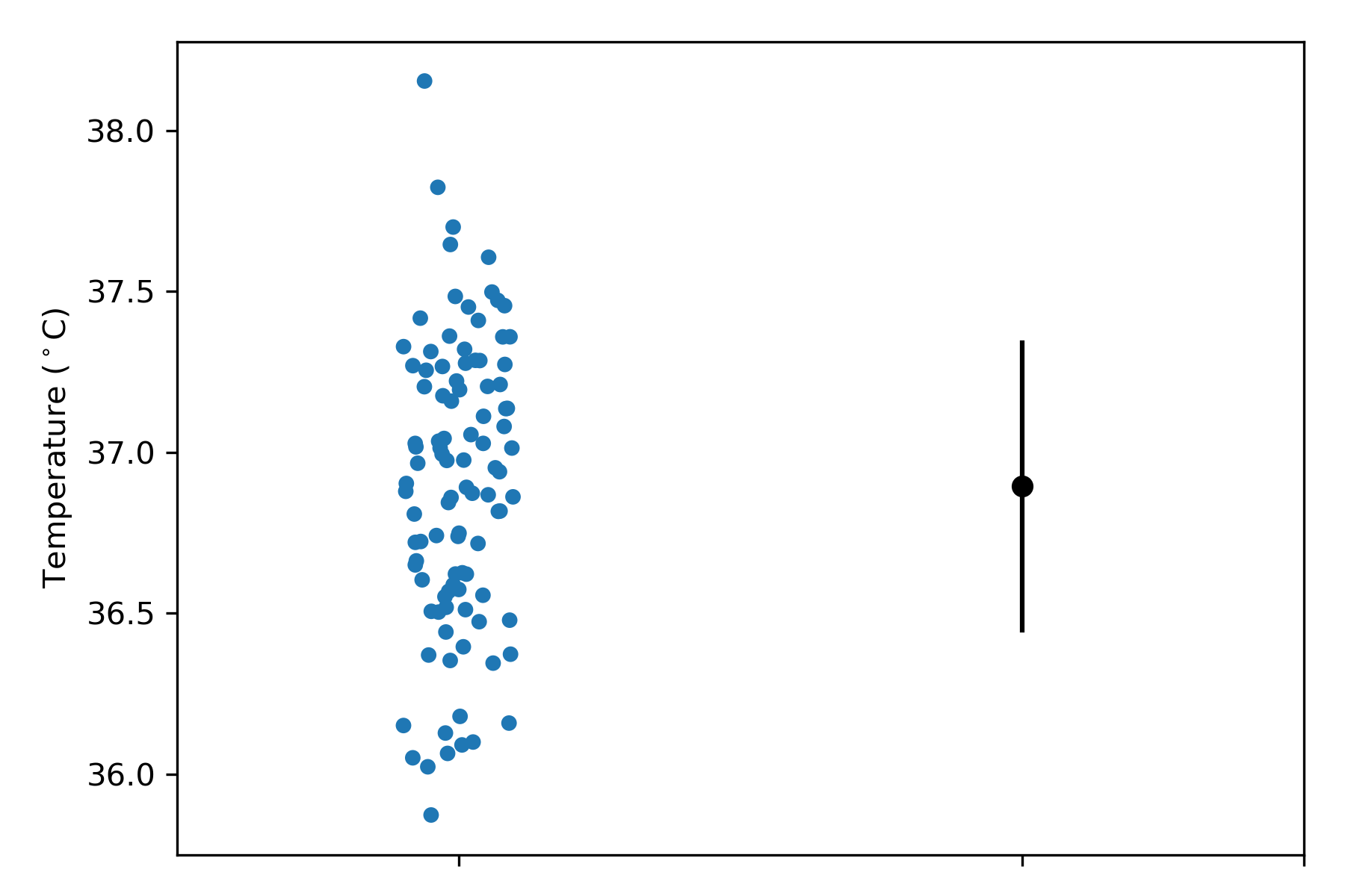
Approximately two-thirds of observations in a population will lie within the range from the mean – 1 SD to the mean + 1 SD. In Figure 1, we see that roughly two-thirds of temperature values (left) lie within the full span of the error bars (right). The SD quantifies the variability in body temperature; the SD increases as temperature values become more variable about the average temperature (i.e. the spread of temperatures about the mean temperature increases), and vice versa. How is the SD calculated? To do so, we need to know how far each data point lies from the mean, add up these deviations, and average them.

Simply adding the deviations won’t work because positive deviations will cancel out negative deviations, causing the average deviation to be zero. To fix this problem, the standard deviation is calculated in this way:

1. Calculate the mean (i.e. the average value).
2. For each data point, calculate the difference between itself and the mean.
3. Square each of these differences.
4. Add up the squared differences.
5. Divide the sum of squared differences by (n – 1), where n is the number of data points – the number obtained is the variance, expressed in squared units of the measurement.
6. Take the square root of the variance; the number obtained is the standard deviation, expressed in units of the measurement.

Squaring the differences stops positive and negative deviations from cancelling out. Taking the square root of the variance expresses the value in units of the measurement (not squared units). Mathematically, the SD is calculated as:

Where represents a single data point, and is the mean.

Why divide by ? This denominator is used to calculate the sample SD, which is the best estimate when a single sample is used to estimate the population SD. The value is known as the degrees of freedom, explained here. In the body temperature example, the variance is 0.17 deg C squared, and the standard deviation is 0.41 deg C.

The SD is one of the most common ways to quantify scatter. Other ways are:

• Coefficient of variation. This is the . If the coefficient of variation is 0.25, this means the SD is 25% of the mean. The coefficient of variation is useful for comparing scatter in variables measured in different units.
• Interquartile range. We could divide the data into 4 percentiles such that the 25th percentile is a value below which 25% of all data points lie. The interquartile range specifies the range of values between which 25-75% of all data points lie. The interquartile range is used when data are skewed.

Summary

The most common way to quantify scatter of continuous data is with a standard deviation. About two-thirds of observations in a population lie within the range from the mean minus 1 SD to the mean plus 1 SD.

Does the standard error of the mean (SEM) quantify scatter in data? This post explains why it does not.

Other variables used to quantify scatter include the coefficient of variation and the interquartile range. The most useful way of judging how variable data are is to see individual data points plotted in a graph.

Next, we will investigate what a Normal distribution is.

References

Motulsky H (2018) Intuitive biostatistics. A nonmathematical guide to statistical thinking. 4th Ed. Oxford University Press: Oxford, UK.